Draft for review. This is a complete draft under active revision. It may contain internal verification markers and editorial notes that will be removed in a final version.
Downloads: Markdown source · PDF · Revision history
Race and Ancestry: Complete draft — under review
1 Introduction
Some today and in the past have made much of race. Whenever possible, arguments for their position are made from the latest scientific reasoning of the day or “the light of nature.” What does the light of nature have to say about race? This paper will examine the answer to that question. The question in particular will be answered in response to the claims of scientific racists and hereditarians (also now sometimes labeled human biodiversity (HBD)). These groups sometimes also identify as “race realists.” I will often use the terms interchangeably throughout this paper.
As suggested by the phrase “light of nature,” this paper is particularly addressed to Christians, especially Reformed Christians. Most of what I present in this paper is independent of that perspective, but I will occasionally make use of that perspective in argumentation, and it has shaped some of the topics I chose to address. For my Creationist readers, I would additionally note that this field is filled with evolutionary theory on both sides. However, the evidence relevant for my conclusions has to do with “microevolution,” and the mechanisms for genetic change in a population are well-established observational science that mainstream modern Creationists would admit.
We will see in this paper that the light of nature shows: 1) There are no biological divisions corresponding to race as it is commonly understood or as it has been scientifically defined—the biology does not divide into races. 2) Race as a category captures very little of the biological variation that does exist and actively misleads about genetic relationships. Statements 1 and 2 are what is meant when scientists and others say “race isn’t real.”1 3) Ancestry has a foundation in biology and can be determined by genetics studies (with limitations), but ancestry and race are fundamentally different concepts with distinct causes and effects and distinct ways of conceptualizing the world, though often confused with each other because of their correlation to each other. 4) While populations do differ genetically in the frequencies of genetic variants, these differences are small, and there is no evidence they produce meaningful differences between groupings of people corresponding to race. Hereditarians claim that observed differences in intelligence and social outcomes between racial groups are caused by genetic differences between those groups. The evidence examined in this paper shows that the genetic differences between populations are far too small to produce such effects, that the specific kind of natural selection that would be required to produce them has not occurred, and that there is positive evidence against its occurrence. It remains possible in principle that genetic factors contribute a small amount, but the range of plausible genetic contribution is far too small to explain observed gaps and is as likely to favor one group as another.
By “meaningful” difference in the thesis above, I am speaking of differences in things that are important to a man as he is made in the image of God, such as intellect, morality, and rule. By contrast, I consider differences in skin color and body shape to not be meaningful. The hereditarian claim, specifically, is that observed differences in these traits between racial groups are substantially caused by genetic differences between those groups. The opposing position, sometimes called environmentalism in this context, holds that group differences are primarily the product of environmental factors—differences in education, income, historical circumstance, and the like. Both sides generally agree that within any given population, both genes and environment contribute to individual differences in traits like intelligence; this is well-established and is not in dispute. The debate is about what causes the differences between groups. Hereditarians further hold that intelligence is what IQ tests measure and that the gaps in IQ scores between racial groups reflect innate genetic differences.
The answer to this question may be shocking, even for those who do not adhere to scientific racism. Most, including myself before this study, likely assume race to be a biological reality as a matter of common sense that only the woke would deny. The light of nature is a genuine source of knowledge, but common-sense observation is only one part of it, and it has never been self-interpreting. As so often happens, scientific study refines and nuances what common sense observed—which perhaps we might have seen if we had paid closer attention—and in doing so, seemingly goes against our intuitions. Consider two familiar examples. Common-sense observation tells us that foul air causes illness and that heavy objects fall faster than light ones. In both cases, the observation tracked a real correlation—people near swamps really did get sick more often, and a rock really does hit the ground before a feather. But careful investigation refined these observations into a deeper understanding and, in doing so, overturned the original causal stories. The air near the swamp really was involved, but it was not the smell that made people sick; it was the microorganisms carried in it. Heavy objects really do tend to hit the ground first, but not because weight makes things fall faster—gravity accelerates all objects equally, and what we observe is the effect of air resistance, which slows lighter objects more than heavier ones. Remove the air, and a feather falls as fast as a hammer. In each case, the common-sense observation was real, but the causal story common sense told about it was wrong—and closer attention to the observations themselves, such as the sailor who falls ill far from any swamp or two cannonballs of different weight that land together, might have revealed the problem before the full theory arrived. Sometimes closer observation can even offer a preview of the true answer, as we will see when we examine what common sense, carefully attended to, shows about the distinction between race and ancestry.
The hereditarian’s appeal to what “everyone can see” about racial difference is in this same category: it mistakes the correlation of race with observed outcomes for evidence that race causes those outcomes. This point must be emphasized, because there is a form of argument—common among hereditarians—that treats correlation, whether from personal experience or data sets, as causation. If we are interested in the causes of things, we cannot rely merely on correlations or experiences. The careful investigation presented in this paper shows that the actual causal picture is quite different from what the hereditarian supposes, more interesting than what has been assumed to be the reality, and more consistent with the biblical testimony of human unity.
In the interest of giving a full picture of what the light of nature shows, I will demonstrate race to not be a biological reality. However, holding to a biological foundation for race does not necessarily entail the various claims of scientific racists about the differences between races. Likewise, there being no biological foundation for race does not necessarily entail there are no meaningful differences between socially constructed groups: it is a logically distinct question, though as will be seen, the lack of biological foundation for race conditions our expectations about group differences, and it helps address questions of kinship that these groups sometimes care about.
Much of this paper is an outline of the evidence summarized by Alexander Gusev, a Harvard geneticist, and I will frequently cite his work: http://gusevlab.org/projects/hsq/. I direct readers who are interested in delving further into the subject to that page, as well as the author’s substack: https://theinfinitesimal.substack.com/. I think readers will find that Gusev deals with the data dispassionately and with self-consciousness about what is established consensus versus what is speculation, and the page is a trove of scientific papers on the topic.
Readers within my circles may have a concern: is he “woke” or a “Leftist” and therefore his commitments may drive his conclusions? I would simply ask the reader to just consider the evidence he presents, how he presents it with distinction between what is known and what is uncertain, and judge whether the evidence backs his claims.
I likewise recommend the work of the creationist geneticist Dr. Robert Carter at creation.com, whose articles I will also be citing here and there. Carter has engaged the hereditarian case directly: in his review of Nicholas Wade’s A Troublesome Inheritance—a book that argues for meaningful genetic differences between races—Carter went in willing to be persuaded and concluded that “there is not much to support the idea that the genetic differences among people groups are significant in terms of outcomes” [Carter, review of A Troublesome Inheritance, J. Creation 28(3):26–30, 2014]. Carter in his review notes the same facts about human genetic variation that Gusev documents: that there is as much genetic diversity within Africa as in the rest of the world combined, and that cultural and historical factors overwhelm the genetic signal [verify that these specific points are in Carter’s review of Wade]. When Gusev and Carter address the same genetic topics, they reach the same conclusions—two scientists from opposite ends of the ideological spectrum, arriving at the same place because the data leads there. I hope this will further set my reader’s mind at ease that the Harvard geneticist is not letting his precommitments interfere with the examination of scientific evidence but is instead being driven by the data to his conclusions.
Indeed, I would note that the view of race not being a biological reality (aside from the human race), which is perhaps the most surprising claim to my readers, is mainstream modern creation science. Carl Wieland, the founding editor of Creation magazine, reaches the same conclusions in his One Human Family [2011], as do Ken Ham and A. Charles Ware in One Race One Blood [2010; rev. 2018]. It is the official position of both Answers in Genesis and Creation Ministries International. I can also say that I have done what I can to understand the field and read the primary literature relevant to the topic to verify claims, rather than rely on any one source’s presentation, and I can confirm that to the best of my understanding that Gusev is dealing with the evidence correctly and even-handedly.
I should also note on this concern of worldview driving conclusions, especially for those who have encountered the hereditarian and “human biodiversity” arguments and found them initially plausible: the individuals and communities driving the movement are, as a group, no friends of conservative Christian morality. The reader who finds that the evidence in this paper is sound should be happy to part company with them.
Before we proceed, it is worth noting a little history. The modern concept of race predates evolutionary theory by more than a century. Linnaeus classified humanity into four races with assigned temperaments in 1758; Blumenbach arranged five races hierarchically in 1795; Darwin did not publish until 1859 [Hannaford, Race: The History of an Idea in the West, 1996]. Evolutionary theory was then used to supply a naturalistic mechanism for racial hierarchy—the idea that races had diverged over time and evolved to different degrees, with some being “less evolved” and closer to the ape. For more than a century, evolutionary biology provided the scientific respectability for race realism. It was also evolutionary biology, in the form of modern population genetics, that eventually dismantled the biological race concept: the data showed nested subsets rather than distinct lineages, gradients rather than boundaries. That the scientific community followed the evidence away from a position that evolutionary theory itself had seemed to support is a mark of credibility, not of political motivation. And it is a conclusion the theological resources of the Christian faith—common descent from Adam, the image of God shared by all humanity, Paul’s “one blood” (Acts 17:26)—had always pointed toward.
This paper proceeds in three main parts, each addressing a different pillar of the hereditarian case: the claim that genetic clustering data reveals distinct races whose biological differences extend to intelligence, the claim that IQ gaps and crime statistics demonstrate innate intellectual and moral differences, and the claim that the historical record of African civilization independently confirms racial cognitive hierarchy—that Sub-Saharan Africa has always been a mess and uncivilized. Part I examines the genetics: the structure of human genetic variation, how populations differ, why those differences do not correspond to race, and what genetics can tell us about the expected size of population-level differences in complex traits. Part II examines IQ and psychometrics: the nature of intelligence testing, the Black-White IQ gap, what environmental and genetic evidence tells us about its causes, and the adoption, admixture, and cross-national data that test the hereditarian hypothesis directly. Part III examines the historical record of African civilization and shows that the record says something quite different from what hereditarians claim. Additional material—including discussions of interracial marriage, crime statistics, and historical voices who opposed racial hierarchy—is treated in sections and appendices as relevant.
2 Human Genetic Variation – What Biology Shows
2.1 Genetic Variation 101
To discuss differences in race, we must first discuss genetic variation. Alleged biological differences in races are attributed by hereditarians to differences in genetics—human genetic variation. What is genetic variation? What kinds of variation? How is it quantified, especially among different populations, and how is it distributed among man? Answers to these questions are needed to respond to the claims of hereditarians. We first turn to the human genome.
2.1.1 The Gneome
The human genome is made up of the entirety of an individual’s DNA. DNA is made up of sequences of chemicals, called nucleotides. For example, a DNA strand might look like: AAGGTAGC, where the letters A, G, C, and T are abbreviations for these nucleotides. The sequences found in the DNA of modern humans is remarkably the same: each individual’s genome has a DNA sequence that is 99.6% the same as any other. The remaining 0.4% varies between human individuals, which is known as genetic variation.
Consider the following to illustrate genetic variation. One individual might have AAGGTAGC and another might have AAGATAGC—the fourth position is occupied by a G in one genome and A in the other genome, but the other positions have the same letters. The genomes vary in the fourth position: this is genetic variation between these two individuals. The different letters that can occupy a position for a gene are known as alleles: G and A are the alleles, in this example. In general, alleles are the different versions of a genetic feature that can appear in a position of the genome, e.g., different versions of genes, which can be made up of thousands of letters, are called alleles also.
This example considers single-letter differences, known as single nucleotide polymorphisms (SNPs) or single nucleotide variants (SNVs). If only variation due to single-letter differences are counted across the genome, then two individuals will have 99.9% identical sequences of DNA, i.e., only 0.1% of the variation in the human genome is due to SNPs. However, there are also variations in blocks of DNA, known as structural variants. One example is short tandem repeats (STRs; sometimes called microsatellites), where a short sequence of letters is repeated many times (dozens of times), e.g., here is GAT repeated: GATGATGAT. Structural variation is rarer than SNPs, but because structural variants involve blocks of nucleotides, they affect more of the human genome and thereby result in the remaining 0.3% of genetic variation. The figure below summarizes the kinds of genetic variation and shows more examples of structural variation.
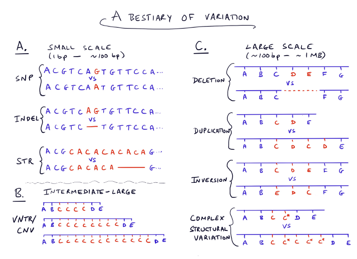
[Pritchard Figure showing kinds of genetic variation at letter level] [Figure from Prithcard p. 36] In Figures B and C, the letters represent large blocks of DNA sequences, rather than the single DNA letters A, T, C, and G.
The genome is very long: 3.3 billion of these letters in length. One copy is inherited from your father, the other from your mother, for a total of 6.6 billion letters to form instructions for the entirety of an individual’s biology. Both copies must be taken together when considering genetic variation. To use my illustration again, suppose that the fourth position on both copies could only have a G, or an A. One individual has the following two copies:
AAGATAGC
AAGGTAGC
The other has the following two copies:
AAGGTAGC
AAGGTAGC
At the variant position (the fourth position), we see that the first individual has AG, while the second has GG. Because in this example the fourth position can only have A or G, there are three possibilities: AG, AA, and GG (AG and GA are the same). This should remind you of the Punnett squares from basic genetics in school: the two copies of DNA produce the different combinations that then eventually express themselves in traits, e.g., eye color, height, or human behavior. Notice that GG and AA each carry two identical copies of the same allele at that position, while AG carries two different alleles. We call a position homozygous when both copies carry the same allele (GG or AA) and heterozygous when they carry different alleles (AG). These terms will matter later: an individual or population with more homozygous positions has less genetic diversity at those positions, and as we will see, this has measurable consequences for health and cognitive traits. However, it should be noted that these single nucleotide differences do not always change what a gene codes for: sometimes they leave the amino acid unchanged (synonymous differences); sometimes they alter the protein sequence (non-synonymous differences).
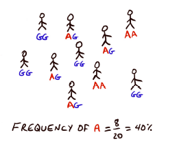
[Illustration of allele frequency] [Figure from Pritchard]
We can look at this position in the genome for a group of individuals and count how many times the alleles occur in the population. This is known as allele frequency. In the population pictured above, the allele frequency of A is 40% (it appears 8 times in the fourth position on either copy of the genome out of a total of 20 times that position appears in a population of 10 individuals) and G is 60%.
Because there are 6.6 billion nucleotides in the genome, we can see from the earlier-cited statistics on variation that there is room for 6.6 million of these letters to differ due to SNPs alone (or 26.4 million, if we include structural variation; these are estimates: closer estimates are 5 million differences due to SNPs alone and 27 million if structural variation is included[). [Numbers from Prithcard and https://www.genome.gov/about-genomics/educational-resources/fact-sheets/human-genomic-variation]] SNPs are the most common source of variation between human genomes. Short insertion/deletion variants such as STRs occur 10 times less frequently than SNPs, and other structural variation occurs 100 times less frequently than SNPs. However, as noted earlier, structural variation causes variation over a larger portion of the genome, and some genetic diseases are attributable to large structural variants. SNPs are useful though for tagging the larger structural variation, including for determining ancestry, so they are the focus for geneticists.
[Structural variation produces continuous ancestry also, see Figure 1d: https://www.nature.com/articles/s41586-020-2287-8]
[Gene info: https://www.genomicseducation.hee.nhs.uk/genotes/knowledge-hub/gene/]
Although the human genome is large, surprisingly, only 1–2% of it encodes information for building proteins, i.e., are genes that have a direct biological impact. About 10% regulates protein production, i.e., regulates the expression of genes—controlling when, where, and how strongly genes are turned on or off. The remaining ~90% is non-coding. Some portion of this non-coding sequence may have structural or maintenance roles that are not yet fully understood, and the fraction that is truly functionless remains an active area of research.2 The arguments in this paper do not depend on assuming non-coding regions are functionless; they depend on the distribution of human genetic differences across the genome, regardless of which regions turn out to be functional.
2.1.2 Recombination
We noted above that the genome comes in two copies: one inherited from your father, one from your mother. In fact, the genome is organized into 23 pairs of chromosomes, with one member of each pair coming from each parent. All the genetic variation we have been discussing—SNPs, structural variants, genes—is distributed along these chromosomes.
Everyone knows that you pass on 50% of your DNA to your children. But which 50%? If each chromosome were passed on intact, then the chromosome your child receives would contain DNA from only one of your two parents—one grandparent—with no contribution from the other. But this is not what happens.
During the production of eggs and sperm, a process called recombination occurs: the two copies of each chromosome are brought alongside each other, and segments are broken and swapped between them. The result is that the chromosome you actually pass on to your child is a patchwork—a mosaic of DNA from both of your parents. [Figure: Illustration of recombination during meiosis, showing homologous chromosomes exchanging segments. A figure from the Pritchard textbook or a standard genetics textbook would be ideal here; see also Coop’s illustrations at gcbias.org.]
This has several important consequences. First, each chromosome pair in your child (with one exception: the X and Y sex chromosomes) contains contributions from all four grandparents, not just two. On average, an individual inherits 25% of their DNA from each grandparent, but because the points at which recombination occurs are largely random, the actual amount from each grandparent varies. Some grandparents may contribute somewhat more, others somewhat less [Coop, “How much of your genome do you inherit from a particular grandparent?” gcbias.org, 2013, https://gcbias.org/2013/10/20/how-much-of-your-genome-do-you-inherit-from-a-particular-grandparent/; for simulations, see Bettinger, “DNA Inherited from Grandparents and Great-Grandparents,” dna-explained.com, 2020].
Second, because recombination is random, your siblings receive a different shuffle of DNA from the same set of grandparents. Each child gets a unique mosaic. This is why siblings who share the same two parents can differ noticeably in appearance and other traits—they carry different random combinations of their grandparents’ DNA [Coop, “Genomic variation in sharing between siblings,” gcbias.org, 2014, https://gcbias.org/2014/01/26/genomic-variation-in-sharing-between-siblings/]. Recombination thereby increases the genetic diversity among children compared to what would exist without it.
Third—and this will matter when we discuss genetic studies of complex traits later in this paper—recombination determines how far apart two variants on a chromosome can be and still travel together from parent to child. Variants that are physically close together on a chromosome will tend to be inherited together, because recombination is unlikely to break between them. Variants that are far apart will be separated by recombination more often and therefore inherited more independently. This correlation between nearby variants is known as linkage disequilibrium (LD), and the patterns of LD differ between populations because the specific points where recombination has occurred accumulate differently over many generations. We will return to this concept when we discuss polygenic scores and why genetic studies performed in one population do not transfer cleanly to another.
2.1.3 Genetic Drift
We have discussed the building blocks of genetic variation: alleles, allele frequencies, the structure of the genome. But how do allele frequencies change over time? What causes one population to end up with different allele frequencies from another? Several forces drive such changes: 1) mutation introduces new variants, 2) natural selection favors variants that improve fitness, and 3) gene flow—the movement of alleles between populations through migration and mixing—makes populations more genetically similar to each other by reintroducing alleles that one population may have lost. We will discuss selection later. But there is a fourth force, less intuitive than the others, that we will discuss now: genetic drift. Drift is a tricky concept due to its probabilistic nature, but as with the other forces, it is essential for understanding how population structure arises and why different populations have different allele frequencies.
Recall the concept of allele frequency from the preceding section on the genome: counting a particular allele across both copies of the genome in every individual in the population gives us the frequency of that allele. Suppose we have a population where a particular site has two alleles—call them M and N—and their frequencies are 50% each. The population then has children, but by chance, the children carry slightly more of the M allele than the N allele. Perhaps parents with the M allele happened to have more children, or perhaps the random process of inheritance (recombination and segregation) resulted in more children receiving the M allele. Either way, the next generation now has an allele frequency of, say, 52% for M and 48% for N. The children’s genomes did not perfectly sample the previous generation—this is what statisticians call sampling error.
If we keep track of the M allele’s frequency across generations, we see it drift: perhaps up to 55%, then down to 47%, then back up to 54%. The frequencies wander randomly—–this is genetic drift. Crucially, drift is random with respect to the fitness of the allele: it causes frequencies to rise or fall without regard to whether the variant is beneficial, harmful, or neutral. It will happen regardless of whether the variant has any effect on traits at all.
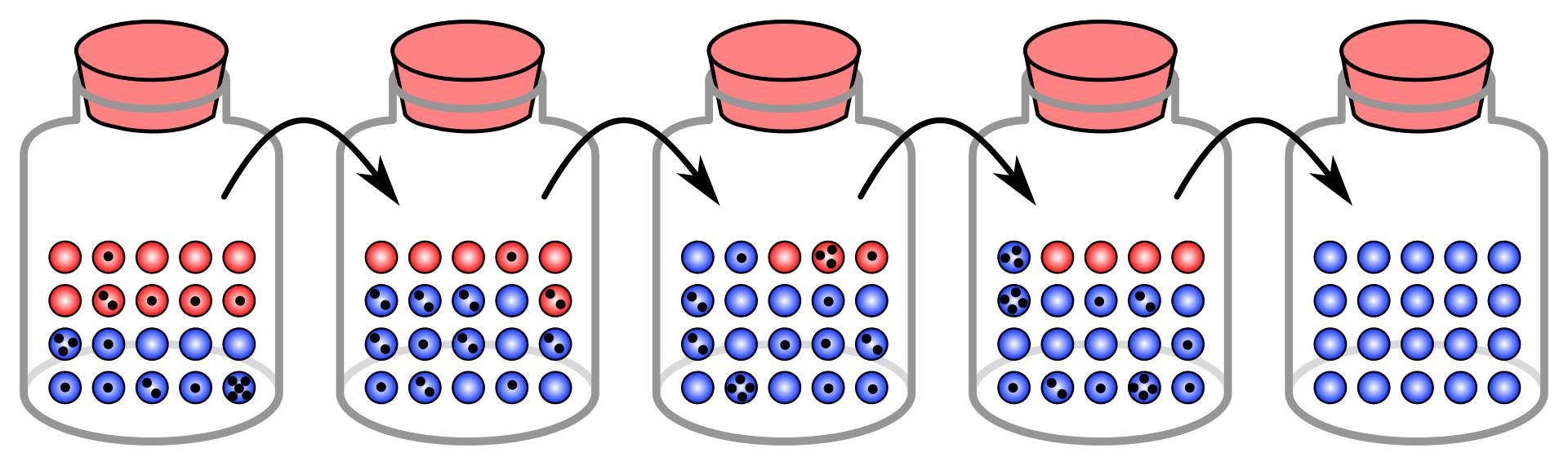
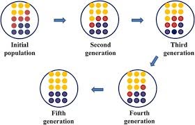
[Figure: Illustration of genetic drift across generations, showing allele frequency fluctuating randomly in a simulated population. Multiple replicate populations starting at the same frequency should be shown, with some drifting to fixation (100%) and others to loss (0%). A standard population genetics textbook figure would work here; see also Pritchard figure or equivalent.]
Now suppose the M allele gains a foothold by chance—say, 60% frequency after a couple of generations. There are now more parents carrying M, which means there is a greater chance that M will be passed on to the next generation, perhaps driving the frequency higher still. It is possible for the M allele to eventually reach 100% frequency, meaning the N allele is entirely lost from the population. This is the ultimate tendency of genetic drift: loss of genetic diversity within a population, as one allele drifts to fixation and the other is lost.
How fast does this happen? In small populations, genetic drift is powerful and fast. Alleles can be lost or fixed quickly, resulting in rapid losses of genetic diversity. In large populations, such as typical human populations, genetic drift is much slower, mostly producing small random differences in allele frequencies between populations.
Bottlenecks are a more extreme example. Suppose a disaster kills most of a population, or a small group separates and becomes isolated from the rest (this is called the founder effect). In either case, the surviving or separated group may, by chance, have allele frequencies quite different from the original population—perhaps 70% M instead of 50%. The next generation starts from this shifted baseline and may drift further still. Bottlenecks are therefore a powerful mechanism for rapidly changing allele frequencies and reducing genetic diversity in a population.
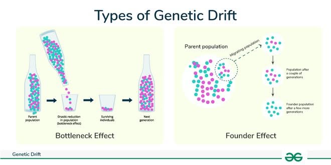
[Figure: Illustration of a population bottleneck, showing a large population reduced to a small group with shifted allele frequencies, followed by population expansion with the new frequencies.]
It is worth noting that the loss of diversity from drift can be partially reversed by gene flow: if individuals from another population, who still carry the lost allele, mix with the population that lost it, they bring that allele back into genetic circulation. Gene flow counteracts drift by making populations more similar to each other.
Why does this matter for our discussion? Genetic drift, combined with geographic isolation and non-random mating (such as marrying those who are geographically nearby), is the primary mechanism by which populations develop different allele frequencies—and therefore the primary mechanism by which population structure arises. As we will see in the next section, the pattern of human genetic variation—with African populations retaining the greatest diversity and non-African populations having progressively reduced diversity—–is precisely what drift and population bottlenecks predict. We will return later to the question of how much of the variation between populations is due to drift versus natural selection—but the reader should keep in mind that drift alone, without any selection at all, is sufficient to produce population structure and allele frequency differences.
2.1.4 How is Genetic Variation Distributed?
One question that arises concerning the variable part of the human genome is its distribution. Are there unique variants to localized regions? Are the variants the same globally and with the same allele frequency? Do some variants show up in one region and continuously change to other variants? The answer to this question is known as population structure and apportionment of variance. This is also the question that must be answered to determine whether there are biological races. The short answer to this question is that: genetic variation is not uniformly distributed. However, surprisingly, most variants are present in all human populations.
Before getting into how genetic variation is apportioned and structured, a brief description of these things. Population structure is a systematic pattern to the genome within a population that results from non-random mating within the population: more specifically, it results in differences in allele frequencies at various loci of the genome for different sub-populations. Non-random mating could arise from a variety of factors. One possibility is assortative mating, in which individuals choose to have children with those similar or dissimilar to themselves, such as when individuals marry those of the same religion (similar) or when taller men marry shorter women (dissimilar). Another (and very common) possibility is geography: individuals mate with those who are geographically local to themselves, especially historically. Forces of change, such as natural selection and genetic drift (discussed in detail in the preceding sections), combined with the non-random mating then leads to genetic distinctions between the sub-populations: their allele frequencies are different.
Population structure should not be identified with race: although race concepts usually include the idea of genetic distinguishability, the presence of population structure does not necessarily indicate a race. For example, there are brown rats in New York City that can be genetically distinguished into uptown and downtown rats, and they will from their own clusters in a graph. These are not separate races/subspecies of rats: they come from one homogenous population likely from Great Britain (as the paper’s analysis states) and are in a city less than 500 years old. The genetic distinctiveness is there, but it is small and not meaningful in a way necessary to think of them as separate races, even intuitively. These are not separate races of rats or highly genetically distinct from each other (they are in the same city!), but this is an example of population structure: non-random mating (and genetic drift in this case) resulted in genetic distinguishability [https://onlinelibrary.wiley.com/doi/abs/10.1111/mec.14437]. Population structure occurs all over the place: so long as there is non-random mating in a population, it will appear. I will show some more examples of this later.
The deeper point is that genetic distinctiveness between populations is not, by itself, sufficient for those populations to constitute races. Population structure—and therefore genetic distinguishability—arises wherever non-random mating occurs, which is nearly everywhere. What biological race concepts require beyond mere distinctiveness—how much private variation each group must have, what kind of branching structure the data must show—is precisely what the biological models of race attempt to specify. We will examine those models shortly and test them against the data.
[[article on genetic distinguishability arising from assortative mating on religion in the Levant: https://www.ibcsr.org/index.php/institute-research-portals/spirituality-and-health-causation-project/560-how-religion-shapes-genetics]]
As for the apportionment of genetic variation, the goal is to figure out how much of the differences in the genome (as measured by proportion/percent of statistical variance [[maybe conceptually explain what this is in footnote]]) are due to various factors.
As for the apportionment of genetic variation, the goal is to figure out how much of the differences in the genome (as measured by proportion/percent of statistical variance [[maybe conceptually explain what this is in footnote]]) are attributable to various groupings. For an example of how this works in order to clarify the idea, consider income variation across the United States. An economist might find that 80% of the variation in income is found within states and only 20% is found between states. Note that the word “due to” here means “attributable to:” this is a description of where the variation is located, not a causal claim that state boundaries cause income to differ. That is, most of the differences in income are found among individuals living in the same state, not between one state’s average and another’s.
[[Note: consider moving example to heritability section. For an example of how this works in another context (variation in a trait, rather than the genome) in order to clarify the idea, consider height differences in a hypothetical population. A scientist wants to figure out: What are the differences in height due to? From study, the scientist finds out 30% of the differences are due to nutrition, 60% are due to differences in genetics, and another 10% are due to differences in exercise. Note that the word “due to” here means “attributable to:” 60% of the variation in height tracks with genetic differences. When genetics and environment are independent of each other, this decomposition cleanly separates causes. When they are correlated or interact with each other—as they often are for real traits—the partition becomes ambiguous, because the portion of variance that involves both genetics and environment can be allocated to either one depending on modeling choices. We will examine this complication carefully in the section on heritability.]]
The first surprising fact about the distribution of genetic variation is that 85% of the SNP variation is due to variation of individuals in a population. This means that 85% of the 1% of the human genome that differs between individuals due to SNPs is attributed to variation within populations, rather than between them, which means most genetic differences are found among individuals within a single population rather than between populations. Another way to think about it: if the variance due to population differences were removed (equalize the average values of a population, e.g., for height differences between men and women, set the average heights equal to each other), in a population, there would still be 85% of the original variation remaining accounted for by individual differences in the population. Only 15% of the variation is due to the variation between populations on different continents. This 15% can further be subdivided into: 5% is due to variance between populations on the same continent and 10% is due to continental variation. That is, only 10% is due to what roughly corresponds to what most race scientists think of as “race”.
This was famously found by Lewontin in the 1970s when investigating blood groups, but these numbers continue to be replicated by various means of calculation: 85-90% of variation is found within any population and the remaining 10-15% is found between continents. If looking at microsatellites, 93% of microsatellite variation is found within a population, 5% is due to continents (i.e., “race”), and 2% between populations on the same continent. [[Rosenberg]: https://pmc.ncbi.nlm.nih.gov/articles/PMC3531797/]
A metric known as Fst formalizes this result. Fst compares the genetic similarity of a subpopulation relative to a total population (more specifically, it measures how much two random alleles from a subpopulation are more similar than when drawn from the total population). This metric essentially captures how “in-bred” a subpopulation is relative to a total population. This functions exactly as “in-bred” would suggest it does: those who are related by a direct familial relationship have much more similar genomes than two genomes of unrelated people, and the more in-bred a population is, the less genetic diversity there is in the population. Fst ranges from 0 to 1. Low values of Fst indicate that two populations are more similar; high, more different. Fst can also be interpreted as the amount of variation attributable to the differences in the subpopulations (i.e., the proportion of variance attributable to the subpopulation label). For populations on different continents (a “continental race”), Fst = 0.15, which is the formal expression of the same 85/15 split described above. This 85/10/5% split has been confirmed time and again by various methods of calculation and of quantifying genetic variation.[[citations]]
We can also see this pattern concretely by looking at individual genomes and counting differences. Genetic diversity is understood to mean more possible allele combinations, e.g., maybe at some site in the genome a population is stuck with GG, whereas a diverse population might have GA, GG, or AA as possible combinations at the site. For this to happen, individual genomes must have unmatching alleles, e.g., GA, at more sites—if they were all the same, e.g., GG at a site, then there are fewer probable possibilities that offspring of that individual can have at that site, especially if their partner is also GG. The degree to which an individual genome has unmatched alleles at sites is known as heterozygosity.
The heterozygosity of individual genomes of various populations are shown below [[citation]]. Notice how individuals from African populations exhibit greater heterozygosity/genetic diversity in their genome. We will return to this point later.
We can also quantify differences between populations by simply counting the genetic variants between individuals in different populations. The result is below. [[citation; gusev]] Note that there are more differences between individuals from an African population (Yoruba) than between an African (Yoruba) individual and a French individual. This again shows greater genetic diversity in African populations and illustrates the 85/15 result concretely: there is more variation within a population than between populations.
In relationship to the question of apportionment of genetic variation, there is also a question: where can the genetic variants be found? It turns out that most of the common SNPs [[check; SNP only?]] are found in all continents with the next largest share of the SNPs being shared by most continents. There are relatively few variants that are private to a population. Rare variants are more likely to be private to a population. See the figure for a chart on global genetic variation. [[Get numbers]; [maybe this but it doesn’t align with the figure I cited? https://elifesciences.org/articles/60107]]
<https://www.nature.com/articles/nature15393; visualizing human genetic diversity with pie charts on global map>
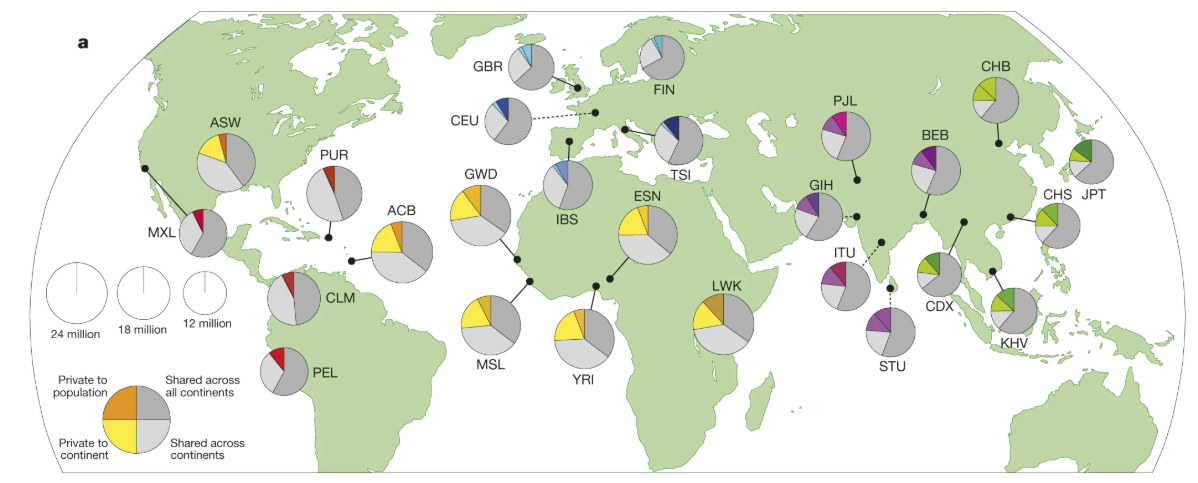
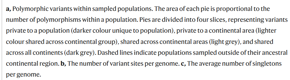
[Useful: Maybe cite: https://james-kitchens.com/blog/visualizing-human-genetic-diversity]
What does this mean? It means that 1) most of the common variants are found in all populations—most alleles are present in all populations, and 2) there is more variation among individuals within a population than between populations. It is not that there are common private alleles to a continent that identify a population to belong to that continent—private alleles are rare—but rather the frequency of certain alleles differs in different populations. These differences are extremely tiny and require looking at many sites in order to match a population to its continent. Moreover, genetic variation is largely continuous with small discontinuities at geographical borders such as mountains or oceans (just 1-2% of the microsatellite variation). [[Rosenberg 2005]]
Thinking about race as a continental population (a population that spans most or all of a continent), this means that there is more genetic variation among individuals within a race than there is between races. Two individuals within a race may genetically vary more from each other than they may vary from an individual from another race, depending on what sites in the genome are looked at (true for a “typical” location, i.e., most locations, not, e.g., locations such as those that give rise to different skin colors)! This is a surprising finding, due to the global distribution of the human population, and it contradicts what classic race scientists thought they would find—vast genetic variation between races and low amount of genetic variation within a race, as I will explain with more detail soon.
2.1.5 Genetic Ancestry
Before we investigate race, we must understand genetic ancestry. Genetic ancestry is the quantification of the blocks of the genome that has been inherited from a recent population (using a modern population as a proxy for that population). It quantifies how much of the genome has been inherited from various populations of interest. Note that genetic ancestry is a relative measure: individuals are more or less similar to each other and to reference populations.
Note also from the definition: there is no access to ancestral populations; the genome is compared to modern populations. Because of this, statements about genetic ancestry are actually statements about the genetic similarity of individuals to modern reference populations. The idea is that genetic similarity is used as a proxy for genetic ancestry. There are obvious limitations to this assumption, including the (incorrect, as we will see later) assumption that the ancestral populations have not moved. This means: we cannot know the actual genetic ancestry of anyone. Not at least, by current methods.
This gap between what genetic ancestry claims to measure and what it actually measures has led population geneticists to recommend replacing ancestry language with explicit statements of genetic similarity. Coop puts the point directly:
“As a field we should move away from genetic ancestry labels and towards simple statements of genetic similarity:”This sample/haplotype is genetically similar to the XX sample set (in comparisons to YYY samples using ZZZ metric)” is much closer to how population genetic methods can be used to provide genetic sample descriptors. For example, “Graham is genetically similar to the GBR 1000 Genome samples (on the first 10 PC)” rather than “Graham has Northwestern European genetic ancestry”. The former sounds a little more awkward, but that awkwardness reflects the truth of how these labels work and comes with many fewer built-in assumptions and pitfalls” coop.
This may seem like a merely technical distinction, but it has real consequences for how ancestry results are interpreted. The connection between genetic similarity and geographic ancestry rests on an assumption that is usually invisible: that the people living in a region today are genetically representative of the people who lived there in the past. At a continental scale, this assumption holds roughly—if large segments of your genome are similar to modern West African populations, you very likely have recent West African ancestry. But at finer geographic scales—individual countries, sub-regions—the assumption begins to break down. Ancient DNA research has shown that many regional populations have been replaced or substantially reshaped multiple times within just a few thousand years. Your genetic similarity to modern Irish people may reflect not Irish ancestors specifically, but a common source population elsewhere in Europe from which both your ancestors and the modern Irish descend. The difference between “your ancestors lived in Ireland” and “your relatives live in Ireland” is not a pedantic quibble—it reflects a genuine gap in what the data can support. Coop et al. lay out the full scope of this problem:
“Most customers of ancestry testing companies are not concerned about technical distinctions between genealogical ancestry, genetic ancestry and genetic similarity. And certainly, genetic similarity can be informative about genetic ancestry on a broad temporal and geographical scales. For example, if segments of your genome are found to be similar to individuals from particular continental groups (”European”, “African”, “Native American”), it is very likely that you have genetic ancestry from those groups in the past few hundreds or thousands of years. However this masks important caveats. Implicitly here we are making use of non-genetic information, for example historical information about population and group continuity in these regions. The geographical connection between ancestry and genetic similarity becomes less clear as we move to more recent or finer-scale structure. For example, at sub-continental scales we are often much less confident about the continuity of populations over the past few thousand years. Emerging evidence from ancient DNA emphasizes discontinuity, with many populations experiencing multiple episodes of replacement over the past few thousand years [15]. As a result, some of your genetic similarity to present-day individuals in a particular country may derive from shared ancestry tens or hundreds of generations ago in a different part of the world. Describing fine-scale population structure in terms of ancestry (“your ancestors lived in Ireland”), rather than relatedness (“your relatives live in Ireland”) underestimates the contribution of migration to human demography.” [<https://pmc.ncbi.nlm.nih.gov/articles/PMC7082057>]
What this means concretely: when an ancestry test reports “20% Irish,” it is really saying “20% of your genome is genetically similar to our modern Irish reference panel”—not that 20% of your ancestors lived in Ireland. Coop’s point is that the field has been conflating two things that come apart at fine scales: similarity, which is a statement about the data, and ancestry, which is a historical claim about who lived where.
The upshot is that genetic ancestry, properly understood, is a measure of genetic similarity to reference populations—and genetic similarity is what produces the clustering patterns that population geneticists call population structure. Individuals with similar genetic ancestry cluster together not because they share some racial essence but because they share more allele frequencies with each other and with certain reference populations than they do with individuals from other clusters. The clusters are real patterns in the data, but what they capture is relative genetic similarity—not membership in a biologically discrete group. This is the framework we need in order to evaluate whether genetic clusters correspond to races.
Genetic ancestry can also be interpreted as a statement about the geographical distribution of one’s ancestors: those who are genetically similar to each other had a similar geographical distribution of one’s ancestors at each point of time. It can also be thought of in terms of lines of ancestry going through the family tree, thereby relating it to the concept of genealogical ancestry. Some ancestors appear more times in the family tree than others, since there are more paths to reach the ancestor through the tree. Some descendants may have an ancestor appearing more times in their tree than other descendants. Those ancestors that appear more times in the family tree are more likely to have passed on chunks of their genome to you, and so those who have similar ancestry have similar frequency at which ancestors appear in the tree. (Coop, https://arxiv.org/pdf/2207.11595)
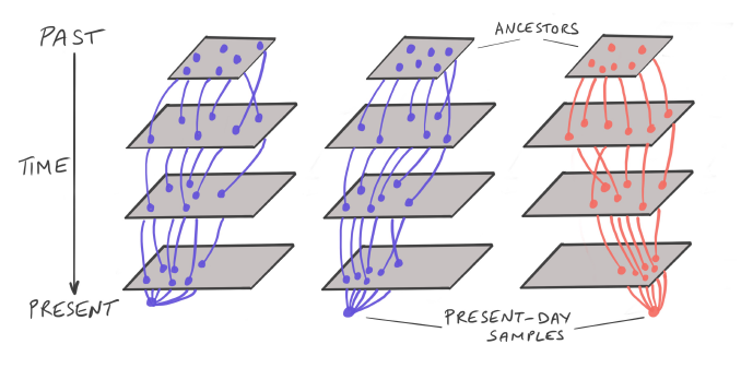
[[Pritchard] illustration of ancestry tree and genetic distribution}
Genetic ancestry is distinct from genealogical ancestry. Due to the way inheritance works—whole blocks of the genome are passed on or not, rather than individual letters being blended—there are exponentially more genealogical ancestors than genetic ancestors. You have 2 parents, 4 grandparents, 8 great-grandparents, and so on; by 10 generations back you have over 1,000 slots in your family tree, and by 20 generations back over a million. But your genome is finite: it contains only so many blocks that can be traced to distinct ancestral sources. Some of your genealogical ancestors—people who genuinely are in your family tree—contributed nothing to your genome. This begins happening as early as five to seven generations back [Coop, “How many genetic ancestors do I have?” gcbias.org, 2017, https://gcbias.org/2017/12/19/1628/; Carter, https://creation.com/review-swamidass-the-genealogical-adam-and-eve; https://creation.com/inbreeding-and-origin-of-races]. In fact, only about 1,000 individuals have contributed genetic material to any given person’s genome [Coop 2017].
The implications are striking. Your genealogical family tree expands so rapidly that within a surprisingly small number of generations, your ancestors span an enormous range of the population. Coop illustrates this concretely: going back just a few hundred years, the number of slots in anyone’s family tree exceeds the total number of people who were alive at the time. The only resolution is that the same individuals appear in multiple slots—your family tree is not a tree at all but a tangled web of overlapping lines. The further back one goes, the more the trees of any two people overlap, until eventually every person alive at some point in the past who left descendants at all is an ancestor of everyone alive today [Coop, “Our vast, shared family tree,” gcbias.org, 2017, https://gcbias.org/2017/11/20/our-vast-shared-family-tree/; “Your ancestors lived all over the world,” gcbias.org, 2017, https://gcbias.org/2017/11/28/your-ancestors-lived-all-over-the-world/; for the mathematical treatment, see Chang, “Recent common ancestors of all present-day individuals,” Advances in Applied Probability 31 (1999): 1002–1026 [verify]]. Due to the vast number of genealogical ancestors, everyone alive today becomes related to everyone else at a remarkably recent point in the past. The family trees of two people intertwine and have much overlap.
This distinction between genealogical and genetic ancestry will matter in two places later in the paper. First, when we examine whether race can be defined as genealogical lineage, we will see that the extensive overlap of family trees across populations makes clean lineage-based groupings impossible—the very genealogical connections that seem to define a race also connect that race to everyone else within a few centuries. Second, when we examine admixture studies that attempt to correlate ancestry proportions with IQ scores, the distinction between genetic ancestry (a measure of genetic similarity to reference populations) and genealogical ancestry (the actual family tree) constrains how those correlations can be interpreted.
2.2 Race and Ancestry
We are now ready to talk about race. In this section, I will show that there is no natural and non-arbitrary way to biologically divide humans into races. I will deal with the proposed racial schemes and show that they do not work. I will also show that race captures little biological information, and I will show how ancestry is a different concept from race and how it allows us to accurately capture biological information.
2.2.1 Race and Ancestry Distinguished
While “race” and “ancestry” are not often sharply distinguished, this paper treats them as distinct concepts that behave very differently. Understanding this distinction will be essential for evaluating the hereditarian claims and understanding various phenomena attributed to race. My readers may not yet see why this distinction matters so much; I ask for patience, as the evidence will make its importance clear soon.
Race, as commonly understood and as used in this paper, refers to one of two things. Most often, race refers to a classification of people into discrete groups—white, black, Asian, and so on—based on perceived physical traits such as skin color and hair type, sometimes together with some notion of ancestral origins. This is race as a grouping: a system for sorting people into categories. There is also an older sense of race as a lineage: a line of descent from a common ancestor, as in the biblical usage of the generations of a people. Both senses will be addressed in what follows; in speaking of “race,” I will usually mean it in the grouping sense unless otherwise noted.
Ancestry, i.e., genetic ancestry, we have already defined in the preceding section: the biological inheritance that can be quantified from the genome. The question this section investigates is the relationship between race and ancestry: whether the social categories of race correspond to the biological reality of ancestry, or whether they are fundamentally different in kind. I will give more formal definitions later. For now, these descriptions are sufficient to follow the argument.
One note before proceeding: although I have referred to race as a social category, I do not beg the question by placing “social construct” into the definition of race or assuming race to be merely a social construct. When I call race a social category, I mean only that racial categories are groupings of people that are widely recognized in society; nothing more is implied by the term. Whether those categories also correspond to a deeper biological reality is precisely the question at hand.
2.2.2 The Common-Sense Argument (Before Genetics)
Before proceeding to the genetic evidence, it should be evident by common sense and a bit of inspection into how race is constructed that race is not only constructed socially, but it is plausibly merely a social construct. This section examines two things available to common sense observation: what genealogical descent can and cannot do for defining race—whether one thinks of race as a grouping or a lineage—and how racial categories behave where they are used. Consider the following.
The theological grounding. We all share common ancestry in Adam and Eve and then again with Noah. Almost certainly all of us have common ancestry with Shem, Ham, and Japheth too. Before Babel, Scripture tells us that “the whole earth had one language and the same words” (Gen 11:1), and God himself observed that “they are one people” (Gen 11:6). If a group is living as one people, marriage among them is one of the things they are doing: we would need good reason to believe the opposite. And who else would they marry? There was no other population on earth. To maintain that the three lines remained unmixed before Babel, one must read separation into a text that describes unity, and nothing in the text motivates that reading except the racial conclusion one wishes to reach. And in the first generation, who would the sons and daughters of Noah’s sons marry except their cousins? Moreover, those who hold that marriage should be among one’s “own people” must, on their own premises, grant that the descendants of Shem, Ham, and Japheth were intermarrying before Babel: for they were, by their own admission, one people. There is therefore every reason to believe that all of us have all three of Noah’s sons as ancestors. That being the case, being a “descendant of Shem” or a “descendant of Ham” does not distinguish any living person from any other.
The key genealogical observation. The human genealogy splits constantly—every marriage, every generation produces a new branch. But a split is not a race. To see what is missing, it helps first to notice what the genealogy does supply. Ask how two people are related and it answers exactly: this man is that woman’s son, these two share a grandfather, this line descends from Shem. Relations of that kind can be traced—they are the genealogy’s own material, and no one can dispute them without disputing a fact of descent. Now ask a different question: how far back must two people share an ancestor before they count as one race? Here the genealogy is silent—not because the facts are missing, but because the question is no longer about a relation. It is about a level: about depth. And depth is the one thing the genealogy produces in unlimited quantity and never privileges. It offers every branch point equally. Relations are traced; they are the genealogy’s own edges. But a racial boundary cuts across those edges at a chosen depth, and to fix it requires someone to decide where to draw the line. The genealogy traces relations. It does not set bounds.3 Descent is traced; bounds are set; kinship is reckoned. The genealogy governs the first. It is silent on the second and the third.
What sets the boundary. The ordinary groupings we find in the genealogy divide sharply on this question. Family needs no set boundary: the relations that constitute it—parent, child, sibling—are the genealogy’s own connections. One does not have to settle a question of depth to know who his mother is. Tribe is ordinarily organized by patrilineal descent from a named founder—the tribe of Judah traces to Judah—and that founder and that line are supplied by the tradition itself, not selected from outside by an abstract criterion. But even the tribal boundary is maintained alongside descent by social rule. Jacob declares Ephraim and Manasseh to be his own sons, “as Reuben and Simeon are” (Gen 48:5), and two of the twelve tribes come into being by a declarative act rather than a birth; the daughters of Zelophehad are told whom they may marry to keep a tribal inheritance intact (Num 36)—one legislates a boundary precisely because descent alone will not hold it unaided. Nation is constituted by non-genealogical criteria altogether—language, territory, rule—and Genesis 10 identifies its seventy nations on that basis. Each of these groupings has something that began at its level: a marriage formed a household; a people began living a shared life under a named ancestor; a group settled a land under a common tongue and rule. Convention may name these beginnings—whether to reckon the family through the father or both parents, whether to call it Judah’s tribe or his wife’s—but the convention names an origin; it does not create one.
Race is different. Race, defined by descent, occupies a position none of these does. It requires a set boundary, since “descended from a common ancestor” picks out no group until a depth is fixed. But it conceptually cannot use the things that fix other boundaries. The whole appeal of descent-based race is that it is supposed to unite people across nations, tribes, languages, and polities—to be deeper and more permanent than any of them, and therefore to bind where covenant and citizenship do not. That appeal is exactly what forfeits the external resources. A nation may say: our boundary is not in the genealogy, but it is in our law and our land. Race, on its own account, can say no such thing, because nothing but descent is supposed to constitute it. It therefore needs the genealogy to supply a level, and the genealogy supplies none. Nothing began at the supra-national level that a racial grouping could be the naming of—no common life, no shared tongue, no origin event. And once a boundary is set by convention, one has a grouping defined by depth and nothing more: that the people gathered there form a people at all, or share anything beyond the descent by which they were gathered, does not follow from the definition and cannot be read off the genealogy.4 Some definitions of race will fare better here than others, and in what follows we take the strongest of them in turn; but each will be found either to set its boundary by criteria drawn from outside descent—which concedes that race is a social kind after all—or to relocate its claim in biology rather than genealogy, which is no longer a question common sense can settle and must be tested against the genetic evidence.
But isn’t “nation” just another word for “race” in Scripture? It may seem so: Genesis 10 names nations after men—Asshur, Mizraim, Cush—and traces them through descent. But a nation named for a founder does not thereby consist only of his descendants, and no one supposes every Assyrian was a son of Asshur. Even Israel, the paradigm case, does not work that way in its own founding generation. The nation is named for Jacob, but Judah’s sons were by a Canaanite (Gen 38:2), and Ephraim and Manasseh were by an Egyptian, yet both lines are load-bearing branches of the covenant people. The founder names the nation; he does not exhaust its ancestry. Nations have real descent content—the Cherokee Nation has a genuine descent core while remaining open to others who join by marriage—but descent seeds the nation without exhausting it, which is exactly why nations admit outsiders and race, on its own account, does not. The point here is not to deflate the biblical category of nation. It is to observe that nation is precisely the kind of thing that has a descent-seeded, rule-maintained boundary, and that race, claiming to be deeper than all nations and constituted by descent alone, has forfeited the rule-based resources that make a nation’s boundary workable.
Any definition of race that grounds itself in descent must select a branching point in the genealogy, and if a definition does not ground itself in descent (basing race on skin color, census practice, or social convention instead), it forfeits the genealogical grounding that made race look like a natural kind in the first place. Such definitions are addressed later in the paper. Among descent-based definitions, the sub-arguments below examine proposals for where to draw the racial line, ordered from the weakest to the strongest; in each case we will find that the level is set rather than traced.
These are not idle taxonomic questions. On the basis of racial categories, people have been segregated, excluded from marriage, and denied the duties owed to kin. If race is to bear that weight, it must rest on something more than an arbitrary choice of where to start counting ancestors. Notice also what these applications of race assume beyond the level: they assume that belonging to a racial group carries significance—that it marks a people, generates obligations, or corresponds to inherited differences. The genealogy says nothing about any of this. A branch is a branch; that membership in one should generate obligations or mark biological differences is a claim the genealogy does not make, and it must be established elsewhere—in the text, if the significance is covenantal, and in the biology, if it is biological.
Common descent. If we are thinking of race as a group coming from a common ancestor, with which ancestor do we start? There is no natural place to begin: the genealogy supplies both convergence and divergence as equally real features of its structure. Going up, all lines converge on Noah and on Adam—one race. Going down, every generation diverges into new branches—as many races as there are families. Simply by moving up or down the ancestral tree by one ancestor will include or exclude a vast number of people from one’s racial grouping. Indeed, we have just as much reason from the genealogy to make no division at all: we have common ancestry in Noah and Adam, so we might as well start with them. In that case, there is no need to think in terms of racial divisions on such significant matters as marriage choices. Perhaps there will be a wish to divide the genealogy into races for other reasons, but those reasons are not present in the genealogy itself.
The patrilineal case. If we are thinking of race as a lineage, which line do we draw—the patrilineal, as in the Bible, or the matrilineal, as in other societies? If we follow both, there is no single line but an interweaving maze. The choice of which to follow is yet another boundary set from outside the genealogy. If race is to be defined by tracing patrilineal descent to a common ancestor—grouping together all those whose father’s father’s father traces back to Shem, or Ham, or Japheth or a more recent male ancestor—then an objective grouping can in principle be made. But it is a boundary set upon the human genealogy, not a division the genealogy traces on its own, and its consequences do not match the racial categories anyone actually uses. Under patrilineal descent, a father’s children are always his race regardless of the mother, and a mother’s children are never her race—they belong to their father’s line. When a daughter marries, her children leave her father’s lineage entirely and join her husband’s. These are not the concerns anyone actually expresses about intermarriage, and the resulting categories will not correspond to the racial groupings the hereditarian cares about.5
Moreover, race so defined becomes unidentifiable. One would need to produce a genealogy to determine which group anyone belongs to, and no one possesses such a genealogy. The Y-chromosome (the biological tool most directly suited to tracing patrilineal descent) cannot help. Not only will it only allow tracing the race of males, Robert Carter, examining the Y-chromosome tree under a creationist framework, found nine distinct hypotheses for how Noah’s sons map onto it, with no way to determine which is correct [Carter, “Can we place the sons of Noah on the Y chromosome tree?”, creation.com, 2024]. Carter also observes that his own Y-chromosome haplogroup (R1b), common in Western Europe, is found at high frequency in Cameroon—on the paternal line, his Irish ancestor was more closely related to dark-skinned Central African men than to some of his Irish neighbors [Carter 2024]. The very line that biblical genealogy traces does not track skin color or any visible racial marker. Skin color does not map to common patrilineal ancestry, and as we shall see later, it cuts across racial boundaries. It is driven by geography and varies with latitude rather than with descent, making it an unreliable guide to anyone’s lineage. Neither does geographical origin, due to migrations and movements throughout history and overlap of populations even among the descendants of Noah’s sons, which we shall see later has also been documented in the genetic data. At the end of the day, a genealogy that no one possesses is needed to identify race this way.
The percentage threshold. Perhaps the criterion is proportional: a person belongs to a race if a sufficient percentage of their ancestors come from that group. But which percentage? Fifty percent? One-quarter? One drop of “other” blood? The “one-drop rule” in U.S. history, blood-quantum fractions for tribal membership, and the Nuremberg Laws’ grandparent-counting rules were all historically used, and they conflict with one another. Every threshold is a convention, not a discovery—another boundary set from outside the genealogy.
The deepest split. The strongest response is that the genealogy does have a privileged cut: Noah’s three sons—Shem, Ham, and Japheth—are the first post-Flood branch, and so (the argument goes) the three races are objectively identified.
This response fails for several reasons. First, as noted above, the lines were never clean: before Babel, the descendants of all three sons were living as “one people”—intermarrying, as one people do, without any recorded command, enforcement mechanism, or physical barrier to prevent it. Moreover, even at the very first branch, the three-way division is clean only under patrilineal reckoning. Each of Noah’s sons married a wife (Gen 7:13). The text does not tell us where these wives came from—they may have been closely related to Noah or they may not have been. But this is precisely the point: the three-way partition is defined by the three sons, and each wife, whatever her ancestry, is not one of those three men. Under bilateral ancestry—counting all ancestors, not just the fathers—each son’s children carried maternal ancestry that does not sort into the threefold patrilineal scheme. The clean tree requires ignoring the mothers and following only the patriline, which is a boundary set on the genealogy, not a fact traced in it. See the patrilineal case above for the consequences of that choice.
Second, the text itself picks out nations, not biological clades. Genesis 10:32 says: “from these the nations spread abroad on the earth after the flood.” What the genealogy of Noah’s sons produces is nations—political, linguistic, territorial peoples—and it produces roughly seventy of them, not three. The popular mapping of Ham to Africa, Shem to the Middle East, and Japheth to Europe is not found in Genesis. As Robert Carter has documented, the Table of Nations shows massive geographic overlap among the descendants of all three sons: descendants of Ham settled North Africa but also Anatolia, Canaan, Mesopotamia (via Nimrod), and Arabia; Shem’s and Japheth’s descendants overlap many of the same regions. The Bible says nothing specific about who settled sub-Saharan Africa, and the Table of Nations has no coherent placement for East Asians, Pacific Islanders, or Native Americans [Carter, “Can we place the sons of Noah on the Y chromosome tree?”, creation.com, 2024].
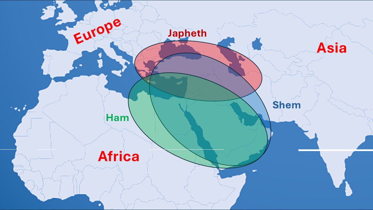
[Figure: Carter’s Table of Nations geographic overlap graphic, from Carter, “Can we place the sons of Noah on the Y chromosome tree?” creation.com, 2024. The visual shows the territories of Ham’s, Shem’s, and Japheth’s descendants overlapping extensively rather than mapping cleanly onto continents.] Carter: “A more realistic map based on the Table of Nations. Descendants of Ham (green) lived in North Africa, but also in Anatolia, Canaan, Mesopotamia, and Arabia, and on the island of Crete. Descendants of Shem (blue) lived in Anatolia, Canaan, Arabia, Mesopotamia, and Persia. Descendants of Japheth (red) lived in Anatolia and Persia, and on the islands of Rhodes and Cyprus. These are just the descendants that are easy to place. There is almost complete overlap among the descendants of the three sons of Noah, but the outlines are highly approximate. Further historical movements would only have continued to blend the lines.”
This geographic overlap means that descendants of different sons were living as neighbors—and people living in close proximity tend to intermarry, even across language barriers, as the biblical examples of cross-lineage marriage confirm. The three-race scheme is not a division that the text mandates; it is one we bring to the text.6
A stronger version of this objection holds that the earliest split, having had the longest time for differences to accumulate, should produce the deepest biological differences along precisely these three lines. This is an empirical claim, and we test it against the observed distribution of genetic variation below; the structure does not recover three coordinate branches. But there is a prior problem. Splitting alone does not tell us whether to think in terms of one race or several. The genealogy splits constantly, and even those who define race by descent treat sub-splits within a line as producing nations and tribes, not new races—on their own account, the branching of Shem’s line into Elam, Asshur, and Aram is not racial. What makes a split racial rather than merely genealogical, on any view of race that requires the groups to be actually distinct, is that the branches stayed apart—that they did not thoroughly remix through intermarriage. This is the one criterion that could convert a set level into a traced one: if the genealogy records which branches separated and which reunited, separation fixes the level without anyone having to set it. Whether lineages kept exchanging marriages is exactly the sort of question a genealogy can answer, and the human genealogy answers it clearly: they did not stay apart.
Entanglement: why the branches never separated. We have seen that what would make the deepest split racial is that the branches stayed apart. The evidence that they did not is both textual and common-sense. The theological grounding above already established the pre-Babel case: the descendants of all three sons were “one people,” intermarrying as one people do, without any recorded command or barrier to prevent it. The mechanism by which entanglement propagates is straightforward: any single cross-boundary marriage introduces ancestry from one group into the other, and the descendants of that marriage carry it forward, marrying within their community and spreading it further with each generation. Even where people mostly marry neighbors, any crossing at a boundary diffuses inward over time. The boundary does not contain it.
The Bible supplies concrete examples of exactly this kind of entanglement at the deepest, most consequential level. Joseph married Asenath, daughter of an Egyptian priest—a union of Shem and Ham through Mizraim (Gen 41:45, 46:20). Their sons Ephraim and Manasseh became two of the twelve tribes of Israel: load-bearing branches of the covenant people, carrying Hamitic ancestry from the very founding of the tribal structure. Ruth the Moabitess married Boaz and became the great-grandmother of David and an ancestor in the messianic line (Ruth 4:13–22; Matt 1:5). Rahab the Canaanite was spared at Jericho and appears in Matthew’s genealogy of Christ (Josh 2; Matt 1:5). These are not marginal figures; they are woven into the line the audience holds most sacred. The boundaries were crossed at the highest-stakes points in the genealogy, and the text treats these crossings not as contaminations to be lamented but as providential acts to be recorded.7
This entanglement defeats not only the three-son division but any attempt to define bounded groups at any scale—whether framed as “meta-races” (large umbrella groups nesting sub-races within them) or as a relative scale of the same phenomenon (every level of division is the same kind of thing as race, with “race” labeling the deepest level). Either version requires the genealogy to branch cleanly, and entanglement ensures it does not: “the family of Japheth” is not a bounded set containing clean sub-sets; it interpenetrates “the family of Shem” because the two families were already mixing before Babel and have gone on crossing ever since.
It may be argued that mixing is insulated by level: that crossings among individuals, families, or even nations are marginal and do not disturb the deeper racial divisions—a foreign wife absorbed into her husband’s people brings no real dilution to the racial stock. But the reply assumes what is in question. Insulation is intelligible where distinct races already exist and contact is marginal at their edges. Before Babel there were no such edges—one people, and the mixing was not at the margins but throughout. And if the proponent grants pre-Babel unity but says Babel created the edges—dispersal, language barriers—the question is whether those edges hold afterward. They do not: every person carries their entire ancestry, so a marriage that looks local joins the whole upstream lineage of each party. A foreign wife’s children carry her ancestry, their children carry it further, and within a few generations it has diffused through the community she married into. There is no membrane at the “racial” level that admits mixing below it while holding the race pure above; local mixing, iterated and given time, is the very mechanism by which racial lines entangle.
It may further be argued that admixture is additive, not dissolutive: large-scale mixing may bring a new race into being, but the two original races persist unmixed alongside it. Notice what this reply does and does not do. It is a claim about what happens to races once one has them; it does not say which populations are the races, and it cannot, since it takes the parental stocks as given. As an answer to the question this section is asking—what fixes the racial level—it supplies nothing. It is worth pausing on anyway, because the position it belongs to does not survive its own rule.8
None of this denies that a bounded group above the family level is possible in principle—a small endogamous tribe or an island community can remain isolated for many generations. But such isolates are historically rare and, as we will see, unstable; and where they exist they define a nation or tribe, not one of the continental “races” the debate is about. The continental-scale groups that racial schemes use are far too large and far too old to have escaped the crisscrossing. The empirical data on gene flow and admixture, which we will examine in the genetics section, confirms and quantifies this common-sense expectation.
The retreat to a gradient. One move remains, and it is the honest one. A proponent who grants everything said so far may give up bounded groups altogether: perhaps there are no races in the sense of sets with edges, but the degrees are real all the same. Some people share ancestors more recently and more densely than others, and that is something the genealogy supplies rather than something anyone imposed.
The premise should be granted. Entanglement dissolves partitions; it does not make everyone equally related to everyone else. But a gradient has no divisions in it. To get races from a gradient, someone must set levels—decide which ancestors to count from, how to weight them, and where along the continuum one group ends and another begins. Perhaps the counting starts at Shem, Ham, and Japheth, and a person’s “race” is determined by how many times each appears in his family tree. But that is the proportional threshold wearing different clothes: the gradient did not escape the level question; it relocated it from “which branch point?” to “which ancestor-count and what percentage?” The same person must set both. And if no levels are set at all—if the proponent insists on a pure continuum with no conventional cuts—then there are no races to speak of, only greater and lesser relatedness, which is precisely the conclusion this section is arguing for. What may follow from degrees of relatedness is a further question, and one the genealogy does not answer: that two people are more or less related is a fact about descent, but that anything follows from it about traits, capacities, or how they should be treated is a claim the genealogy never makes. The trait question we take up in the genetics that follows.
The mixed-ancestry observation. Returning to the idea of mixed ancestry, everyday language already treats ancestry as proportional and continuous rather than falling into a discrete category. Very often, many in answer to “What is your race?” will describe their race as coming from multiple places, e.g., 25% German, 50% Dutch, 10% British, 15% French. Or they will say, “She’s a quarter Cherokee,” “He’s half Italian, half Puerto Rican.” Common sense is showing us that we have a notion of ancestry that does not reduce to a discrete race: indeed, assigning a racial category would discard most of the biological information. The existence of such people (and their self-understanding) is showing us that ancestry and race are different things in practice, and ancestry conceptually is a continuous and proportional quantity.
The social variability of race. Moreover, we can look beyond mere common sense inspection and proceed to see how race has actually been defined. Different nations have different racial schemes based on social preferences for classification, rather than biological taxonomical criteria. For example, in Brazil, race is primarily based on appearance (like skin color): if a family has children with brown skin and white skin, they are considered separate races! The classifications are white, brown/mixed, Asian, indigenous, and black, and sometimes, it was possible to move between classifications via wealth: “Money whitens” capturing the idea that wealth could make one perceived to be or self-identify as “whiter” than their physical features would suggest.9 In a 1976 national household survey, Brazilians given an open-ended question about their cor (color) produced 136 distinct answers; a 1998 survey produced 143 [Telles 2004]. But before that number misleads: 95 percent of respondents used only six terms—branco, moreno, pardo, moreno-claro, preto, negro—and 77 of the 1998 terms were given by exactly one person each [Telles 2004]. What the number shows is not that Brazilians recognize 136 races, but that when asked about race in their own words they reach for shade descriptions—points on a continuum, not fixed categories. And even those six common terms are applied differently by region: a person considered pardo (brown) in Curitiba, in the European-influenced South, may be considered branco (white) in Salvador, in the Northeast [Monk 201610]. No ancestry-based system can produce that result. A biological property does not change with the demographic composition of the surrounding population.
In the U.S., the scheme has changed in every decade: the race question has never been the same from one census to the next [Jones, Jensen, Battle and Marks; Pratt, Hixson and Jones 2015; see also U.S. Census Bureau, “Race and Ethnicity Across the Decades: 1790–2020”]. In contrast with Brazil, the U.S. schemes are often more focused on geographical ancestral origin. Take the changing definition of “black,” for example, which due to how it was defined also impinged upon the definition of “white.” The portion of African ancestry to be considered black would change through time: Virginia moved from one-quarter (1785) to one-eighth (1866) to one-sixteenth (1910) to any trace at all (1924). Louisiana was still at one-thirty-second as late as 1970, and did not repeal that statute until 1983 [Davis 199111]. Most famously, the “one-drop” rule ensured that any hint of African ancestry would cause a person to be viewed as part of the “black” race, and the rule was written into federal census enumerator instructions from 1930 through 1960: “A person of mixed white and Negro blood should be returned as a Negro, no matter how small the percentage of Negro blood” [U.S. Census Bureau 1933, pp. 1398–1399; quoted in Humes and Hogan 2009, p. 117]. See also 1904 instructions at [U.S. Census Bureau Bulletin 8 1933, p. 14 Negroes in the United States]. What this meant in practice: Walter Francis White (1893–1955), executive secretary of the NAACP, had blond hair, blue eyes, and fair skin. He described himself as a Negro on whom none of the traits of his race were visible [White, A Man Called White (1948), p. 3]. He could have passed permanently; he chose to live as Black and used his appearance to investigate lynchings in the South. Both the society and the man agreed on the classification, and the classification had nothing to do with how he looked.12
Were these classification systems due to careful scientific study? Did the changes happen due to better scientific evidence? Brazil’s system is plainly not biological: when money can change your race, biology is not the operative criterion. As for the U.S., four rules from the same page of the 1930 census instructions tell us the answer. A child of a white parent and a Negro parent was to be returned as Negro “no matter how small the percentage.” A child of a white parent and an Indian parent was to be returned as Indian—unless “he is regarded as a white person by those in the community where he lives.” A child of a white parent and any other non-white parent was to follow the non-white parent. A child of two non-white parents was to follow the father—except if one parent was Negro [U.S. Census Bureau 1933, pp. 1398–1399; Humes and Hogan 2009, p. 117]. Four rules for the same biological situation—one parent from one group, one parent from another—with no biological fact distinguishing the cases. The Indian clause defers to community perception by name. And Humes and Hogan, both Census Bureau staff, describe the purpose plainly: the 1930 census used the one-drop rule “to maintain a white category that was as ‘pure’ as possible.” Census Bureau authors writing in 2024 said the quiet part out loud: the underlying purpose of asking about mixed ancestry for the Black population was exclusion, while the purpose for asking similar questions for American Indians was to measure assimilation [Jones, Jensen, Battle and Marks, p. 7].13 Same instrument, two groups, opposite goals, and no biology behind the difference. Today, if someone has some amount of African ancestry but has white skin, they may be considered white, depending on who you ask—perceptual research puts the modern threshold at roughly 60% European appearance, nowhere near one drop [Ho et al. 201114]—but an asymmetry remains: it takes more European appearance to be read as white than African appearance to be read as Black, and the size of that asymmetry varies with which minority group is involved, not with how much ancestry is involved [Ho et al. 2011]. A biological threshold would not care whether the other parent was Asian or Black.
The boundaries have also shifted with geography. From 1977 to 2024, the U.S. federal government classified Middle Eastern and North African (MENA) Americans as White [OMB, Statistical Policy Directive 15 (1977); Humes and Hogan 2009, p. 119]. But MENA Americans were neither perceived as White nor self-perceiving as White: in survey experiments, when a MENA option was offered alongside White, 88% of MENA respondents chose it [Maghbouleh, Schachter and Flores 202215]. On March 28, 2024, OMB revised the standard to add “Middle Eastern or North African” as a separate category, distinct from White—the first major revision since 1997 [Jones, Jensen, Battle and Marks, pp. 20–24]. The official racial category of roughly three million people changed by administrative decision, on the basis of survey research about how people are perceived, with no new genetic information involved at any point.16 Similarly, Dominican immigrants may be classified as indio or blanco at home but as Black in the United States—the same person sorted by different rules in different places, with the rules being cultural inheritances rather than readings of biology [Roth, Race Migrations (2012)17].
It should be clear that these classifications are arbitrary and have no relationship to a serious study of biology or even a serious study of ancestry: racial classification is not even an attempt to accurately capture biological information. Beginning with the 1950 census the Bureau stated that its concept of race “is derived from that which is commonly accepted by the general public” and “does not, therefore, reflect clear-cut definitions of biological stock” [U.S. Census Bureau 1953, p. 3B-4; 1963, p. X; Humes and Hogan 2009, p. 118]. The 2024 federal standard says the same thing more plainly: the categories are “sociopolitical constructs and not an attempt to define race and ethnicity biologically or genetically” [OMB, SPD 15 (2024); Jones, Jensen, Battle and Marks, p. 24]. Should we prefer Brazil’s method of being primarily concerned with phenotype and ability to “whiten” one’s race? Or should we prefer the U.S.’s method and be focused on geographical ancestral origin? Both of these are related to biology, but the reasons to prefer one or the other for racial classification are arbitrary and rooted in social reasons—Brazil with its whitening ideas; the U.S. with its desire “to maintain a white category that was as ‘pure’ as possible” [Humes and Hogan 2009, p. 117]. In the U.S., even a person with 99% white ancestry and features could at various points in history be considered black: what does this have to do with biology when such a person would be more biologically like a typical white man? Blacks in the U.S. have on average 20–25% recent (!) white ancestry [Bryc et al. 2015; Baharian et al. 2016; 1000 Genomes ADMIXTURE of ASW], and yet they are considered black—their own distinct race—without any regard for that fact, especially by scientific racists who I have yet to see consider them to be in any sense their own family or blood beyond their membership in the human race18. A person with four West African grandparents is classified Black under a biological account and a social account alike—such cases carry no information about which account is correct. The cases that tell us something are precisely the ones where the two accounts predict differently: Walter White, the Healy siblings, MENA Americans, Dominicans who change race by boarding a plane. And the mismatch is not exceptional—it is the normal state of affairs, differing only in degree. If 20–25% of the average Black American’s ancestry is European, then mismatch between the racial label and the actual ancestry is typical; what is rare is the mismatch being visible enough to notice. These issues with race as a biological category foreshadow what we will soon see: race is a discrete category that does not accurately capture the proportions of a person’s ancestry and doesn’t care if a person’s genome is more similar to a person who was placed in another distinct racial category.192021
What common sense establishes. What we see, then, from common sense and before looking at genetics:
- The genealogy sets no racial level. Every proposed criterion—the deepest subdivision, a percentage threshold, a specified line of descent—requires a standard the genealogy does not supply. The boundary is set, not traced.
- The one criterion that could have fixed the level without anyone setting it—separation of the branches—is contradicted by the record. Before Babel, one people; after Babel, geographically interleaved nations; at the highest-stakes points in the covenant line, cross-lineage marriage. The genealogy shows entanglement, not separation.
- The retreat to a pure gradient does not escape the level question. A gradient has no divisions in it; to get races from a gradient, someone must set levels—which is the proportional threshold again. And if no levels are set, there are no races to speak of, only continuous relatedness.
- Even a determinate, bounded grouping would carry no significance—no information about traits, capacities, or obligations—without an independent argument that the genealogy does not supply.
- Beyond the genealogy: existing racial schemes are socially variable and discard proportional ancestry. Different societies construct different categories from the same ancestry, and assigning a discrete racial label throws away most of the biological information that ancestry provides.
Given these results, we would suspect that racial schemes do not have a biological reality to them: the categories are socially constructed in origin and lose biological information even where they try to track biology. But common sense raises the suspicion; it does not settle it. We must turn to genetics to see whether the suspicion is confirmed.
What common sense does not yet settle. It remains possible that the observed differences between populations might correspond to a biological reality that, while not readable from the genealogy or from social classification schemes, could be discovered by genetics. Perhaps the genealogy provides no basis for race, but biology does—perhaps the categories, though not mandated by descent, happen to track something real about human variation. It is also true that there have been attempts to define and identify biological races in humans. We now turn to investigate these and see how they compare with the data on genetic variation.
2.2.3 Setting Up the Genetic Test
Before examining the genetic data, we must establish what race would need to show biologically. The point of establishing these definitions and models before presenting the data is to prevent the goalposts from shifting after the results are in. If race is biologically real, we should be able to specify what that means in advance and then check whether the data conforms.
Formal definitions. Gusev presents the following model of the relationship between race and ancestry:
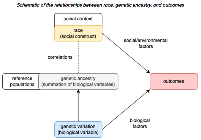
[Gusev model of race and ancestry illustration]
He defines race as: “[T]he social categorization of individuals into groups based on perceived (typically physical) traits. It can be further subdivided into (a) self-identified race and (b) race as perceived by others (naturally these two concepts also interact: people who are told they are a given race will start to perceive themselves as that race). As it is a social construct, race is estimated through self-reporting; there are no ‘biomarkers’ or ‘diagnostics’ for race. Race is often correlated with physical features (e.g. pigment) and, by proxy, with their genetic underpinnings (e.g. pigmentation genes).”
Pritchard writes: “Race categories are socially constructed labels that group people based on features such as ancestral origins, culture, and often physical characteristics such as skin pigmentation and hair type. Conceptions of race and ethnicity vary among countries, and can change through time, but generally have some imprecise relationship with the concept of ancestry.
The term race is not easily defined, but ‘race’ is usually thought of as relating to ancestral origins and physical characteristics.”
These are typical definitions by geneticists. I will note again that we don’t have to define race so that social construct is in its definition and thereby apparently beg the question: just view this as a definition of socially constructed race and see if there is a biological basis for it also. Furthermore, the definition should explicitly include some relationship to ancestry (as Pritchard notes). With these modifications, I think the definition accurately captures what many mean by race. Alternatively, the definition and diagram presented by Gusev can be viewed as a model, and we will see if it fits the data better than biological racial models, or see how this model emerges from considering the evidence.
Biological models of race. - AI gen We are now ready to investigate the proposed biological models of race and compare how they stack up to the pattern of human genetic variation. Do they explain the amount and pattern of genetic variation well? Do they do well at categorizing the genetic differences among individuals or populations?
The essentialist model. The first concept is the essentialist view of race: a race denotes a group of individuals who are genetically distinct from other races, highly genetically similar to each other, and fixed in their genetic differences from other races. There is some overlap on the margins of these races resulting in mixed races. These races are viewed as having formed by branching off and being isolated for a long time. The essentialist view of race largely determines race based on physical characteristics with some ideas of genealogical ancestry also. This is the classic view of race, which became indefensible, and so modern race scientists often go to the second concept of race.
The population model. The second concept is the population concept of race: a race denotes a population that shares genetic variation among its members but has some genetic variation that overlaps with other populations. Crucially, each race-population has its own large share of genetic variation that other race-populations do not have. This is more than mere statistical distinguishability—any two non-randomly-mating populations will have slightly different allele frequencies, as we saw with the Manhattan rats. The population concept requires more: each group has a substantial pool of private variation, enough that the groups are, in a meaningful sense, their own genetic entities with their own character. (A closely related concept is the taxonomic definition of race due to Mayr [Mayr 1969], which defines a race as an aggregate of phenotypically similar populations inhabiting a geographic subdivision of a species’ range and differing taxonomically from other such aggregates. This adds phenotypic identifiability to the population concept but shares the same core requirement: each racial group must possess a substantial portion of its own distinctive variation. Both fail for the same reasons, as we will see.) Furthermore, under both the population and taxonomic concepts, the racial groups are implicitly placed at the same level of classification—African, European, Asian are treated as coordinate categories of roughly equal rank, each with a comparable share of its own variation. This is what Panel B in the figure below depicts: roughly equal-sized circles, each with a large non-overlapping region.
The evolutionary lineage model. The third concept views race as an evolutionary independent lineage—a population that branched off from others and has been developing along its own path, accumulating its own genetic changes through drift, new mutations, and selection, with little gene flow back to the source population [Templeton 1998; Long and Kittles 2003]. Where the population model asks how much private variation each group has, the lineage model asks whether a branching event occurred that produced a pattern where within-group relatedness slightly exceeds between-group relatedness. In practice, this is tested by fitting a branching tree to the genetic data and seeing whether it captures the pattern of relatedness among populations. The Euler diagrams and variant-sharing patterns we examined above are evidence for the tree topology, but the lineage model’s argument is ultimately about the shape of the tree, not about the amount of variant overlap between groups. The lineage concept adds a historical claim beyond what the population model requires: not just that each group has its own pool of variation, but that each group’s distinctiveness reflects a history of independent development after separation. This predicts a tree-like branching structure of human genetic variation, where populations form a clean-branching family tree, each branch having accumulated its own genetic profile over time—similar to how separate species behave after splitting. As with the population model, this implicitly treats the major racial groups as coordinate categories at the same level of classification, each representing its own independently developing branch. We will see that this prediction is directly contradicted by the nested subsets pattern.
Under both the threshold and lineage definitions, genetic differentiation is necessary but not sufficient—both additionally require that the differentiation occurs across sharp boundaries reflecting historical splits, not as gradual change [Templeton 2013]. This means that seeing separation on a PCA plot or identifying clusters in a STRUCTURE analysis establishes genetic distinguishability, but not that the groups in question meet either criterion for biological race. Population structure arises wherever non-random mating exists—between continents, between neighborhoods, between religious communities—and PCA will detect it at every scale. The question is whether the differentiation rises to the level, and takes the form, that biological definitions of race require.
What any of these models predict. If races are biologically real under any of these definitions, the data should show: (a) more variation between groups than within them, (b) largely private variants for each group, and (c) a tree-like or cluster-like structure rather than a gradient. We have already reviewed the data on genetic variation in Genetic Variation 101. Let us now see how these models compare to it.
Note: these are the models that became indefensible. Modern race scientists often retreat to updated definitions—I will address those in the Objections section.
2.2.4 The Genetic Evidence: What the Data Shows
How do these biological models of race stack up to the data?
The 85/15 result falsifies both the essentialist and population models. Based on the apportionment of human genetic variation that we discussed, the essentialist view of race does not stack up at all. Individuals within a population have high genetic variability in comparison to the genetic variability between populations. Furthermore, populations are in a constant state of genetic change (at the least from genetic drift making the allele frequencies fluctuate) and have genetic structure among their subpopulations. Likewise, the population view of race fails since most genetic variation is common among all populations. Both models predicted more genetic variation between groups than within them; the actual result—85% within, 15% between—is the opposite.
The nested subsets model. - AI gen There is a model that does explain genetic variation well: the nested subsets model. All genetic variation is largely a subset of variation in Africa with Africa having the largest genetic variation. Africa, and more specifically sub-Saharan Africa, contains almost all the genetic variation that is worldwide. In the figure below, you will find the different views of race visualized and in panel D is what actual data looks like.
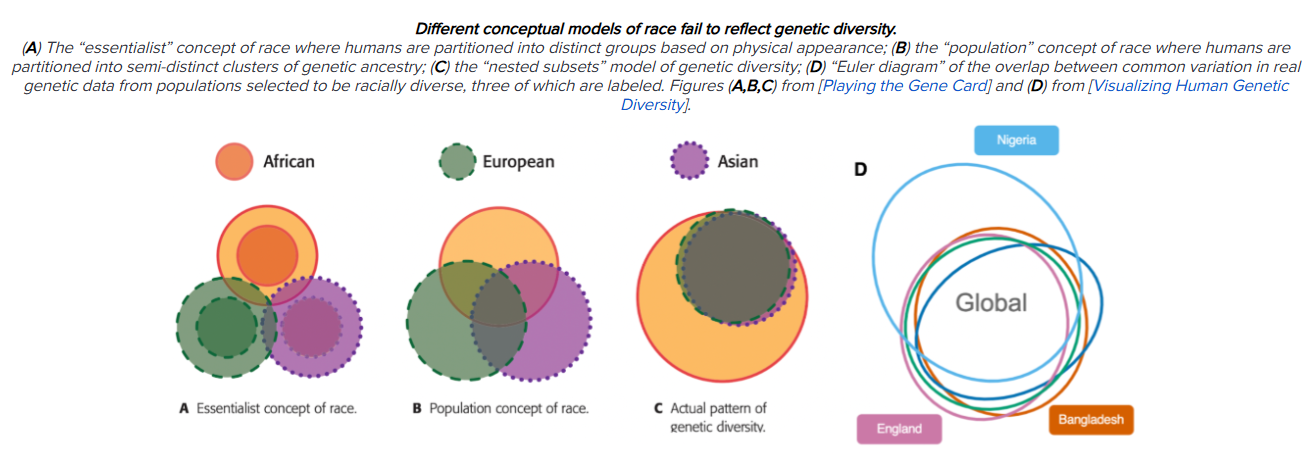
[Gusev figure of race models including nested subsets. Panel D is based on real genetic data from the 1000 Genomes Project, visualized by Kitchens and Coop [Kitchens and Coop 2023, “Visualizing the shared nature of human genetic variation,” Zenodo/GitHub].]
In this figure, panels A through C depict the three race models just described; panel D shows what the actual data looks like. The circles in panel D are Euler diagrams, where each circle’s area is proportional to the number of common genetic variants (those found in more than 5% of individuals’ chromosomes) in that population sample. The overlap between circles represents variants that are common in both populations. Notice that the Nigerian sample’s circle is dramatically larger than those for England or Bangladesh. This size asymmetry is the nested subsets pattern: the African population contains far more common genetic diversity than non-African populations. Compare this to Panel B, the population concept of race, where the circles are roughly equal in size, each with a large non-overlapping region. The actual data looks nothing like that.
The reader may notice that the England and Bangladesh circles extend somewhat outside the Nigerian circle. This does not mean that those variants are absent from Africa. It means they are rare in Nigeria—present at below 5% frequency—but have risen above that threshold in England or Bangladesh through genetic drift after the population bottleneck, through Neanderthal admixture in non-African populations, or through local selection. The dominant feature of the diagram remains massive sharing, with the African sample containing the superset of variation [Kitchens and Coop 2023].
What does this pattern mean for the models of race? The essentialist and population models assumed that each racial group would have its own large share of genetic variation distinct from other groups. The data shows the opposite: most genetic variation is shared across all populations, with African populations containing nearly all of it. Non-African populations’ variation is largely a subset of African variation, plus a small amount of additional variation from post-bottleneck drift and archaic admixture. This pattern—called nested subsets—is fundamentally different from any race model. A race model that fit this data would need to be defined by nested subsets, serial bottlenecks, and extensive admixture—which, as Gusev notes, would be nothing like the conventional use of race. Quoting from Gusev on this point (explaining his figure), who of course assumes out-of-Africa22,
“The early ‘essentialist’ models of race advocated for the partitioning of humans into fundamentally distinct groups based on appearance, with some overlap at the margins to acknowledge ‘mixed-race’ individuals. These models operated under the assumption that human races had undergone substantial divergent evolution and that most genetic variation had fixed to different values between racial groups, leading to observable differences in skin and hair. More contemporary population/ancestry based models of race continue to advocate for partitions between ‘populations’ of individuals but rather than base these partitions on hard physical characteristics, they are based on softer genetic ancestry ‘clusters.’ In truth humans spent most of their evolutionary time in Africa, which included the accumulation of the vast majority of common variation (see 8.3), followed by multiple gradual and complex dispersals and mixtures into other parts of the world. These dispersals involved population ‘bottlenecks’ that increased drift and thereby reduced the genetic variation in the subpopulations, yielding a ‘nested subset’ of populations where most genetic variation present outside of Africa is also present inside of Africa (with non-African populations experiencing a small amount of additional novel variation through admixture with archaic humans). Indeed, using real genetic data from populations selected to be as geographically and racially diverse as possible we see that the observed patterns of genetic variation closely match this nested subset model and have no correspondence to either the essentialist or population-based concept of race (panel D above). Even as an abstraction, race-based models do more to mislead than inform our understanding of contemporary genetic diversity. A model of race that would even remotely correspond to biological genetic diversity would need to be defined by nested subsets, serial bottlenecks, and extensive recent admixture—in other words, it would be nothing like the conventional use of race both historically and today.”
The force of Gusev’s conclusion is worth stating plainly. Both the essentialist model (races as fundamentally distinct types) and the population model (races as discrete ancestry clusters) predicted that each racial group would carry its own substantial body of genetic variation, distinct from the others. What the data actually shows is that one region—Africa—contains nearly all the common variation, and the rest of the world’s populations carry progressively smaller subsets of it. This is not a minor discrepancy that could be patched with a better classification scheme. It is a structural mismatch: the biology does not divide into the symmetrically differentiated groups that any racial model requires. What remains is population structure—real, measurable, and scientifically informative—but not race.
Seeing the subset relationship directly. The figure above shows the overall sharing pattern, but there is an even clearer way to see the subset relationship. Kitchens and Coop performed the following analysis: for each population sample, they identified the variants that are common in that sample, and then asked how many of those variants are also common in the other samples. When this is done, the highlighted sample’s circle completely encircles all the other circles—because nearly all of its common variation is also common elsewhere.
[Kitchens and Coop Figure 4, two panels: one filtered on GBR (British in England and Scotland), showing that nearly all British common variation is shared with the other samples; one filtered on YRI (Yoruba in Ibadan, Nigeria), showing that the Yoruba sample has a larger exclusive area—variation common in Yoruba but rare elsewhere. Static screenshots from Kitchens and Coop 2023; the original figures are interactive and can be explored at https://james-kitchens.com/blog/visualizing-human-genetic-diversity.]
The contrast between these two panels is the nested subsets pattern stated visually. When we look at what is common in England, nearly all of it is also common in Nigeria and Bangladesh—there is almost nothing uniquely common in England alone. But when we look at what is common in Nigeria, there is a substantial region of variation that is common only there and rare elsewhere. Non-African variation is largely contained within African variation, but not vice versa.
Formally testing the models. - AI gen It is also possible to test models of race by fitting them directly to the data on genetic variation and seeing how well they match. If race is a biological phenomenon, a race-like model should match some pattern of genetic variation. Long, Li, and Healy (2009) formally tested a race-like model (the Two-Level Island Model, which operationalizes the race-as-discrete-populations concept) against a nested subsets model (the Expanded Hierarchical Model, which captures the pattern of non-African diversity being largely a subset of African diversity). It turns out that the race-like model fits very poorly, while the nested subsets model fits the pattern of variation extraordinarily well.
The way this test works is straightforward. Genetic distance is a measure of how genetically different two populations are, based on their allele frequency differences: the more their allele frequencies diverge, the greater the distance. (The figures below use two related metrics: nucleotide diversity, which measures how different two randomly chosen DNA sequences are, and a normalized genetic distance derived from it. Both capture the same underlying comparison; the two columns simply show the model fit using different scales.) Each model predicts what the genetic distance between every pair of populations should be. Those predictions are then compared to the genetic distances actually observed in the data. In the scatter plots below, each dot represents a pair of populations; the horizontal axis is the distance the model predicts, the vertical axis is the distance actually observed, and the diagonal line represents a perfect prediction. The closer the dots fall to the line, the better the model fits. The race-like model scatters its predictions badly (R² = 0.38), while the nested subsets model tracks the observed data closely (R² = 0.94).23
[Gusev figure from Long, Li, and Healy 2009, recompiled by Gusev; shows race-like model (top) vs. nested-subsets model (bottom), with tree diagrams, nucleotide diversity comparisons, and predicted vs. observed genetic distance scatter plots]

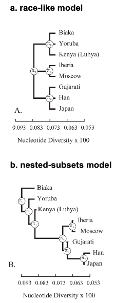
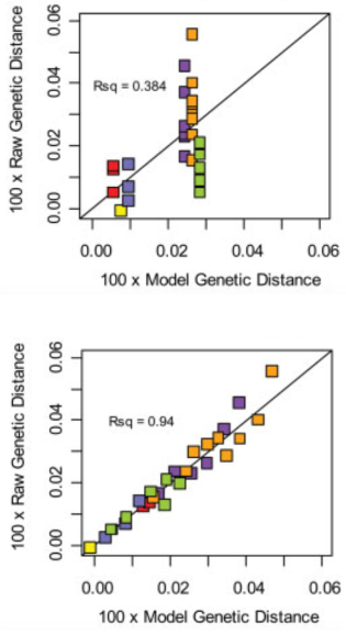
The nested subsets model falsifies the evolutionary lineage model. - AI gen The lineage definition of race requires that the members of a race be more closely related to each other than to members of other races. If African, European, and Asian are each races under this definition, then individuals within each group should be more closely related to each other than to individuals in the other groups. Long et al. tested whether the nested subsets pattern is compatible with this requirement [Long 2004; Long and Kittles 2003; Long, Li, and Healy 2009]. It is not, and the reason is that the nested subsets pattern is asymmetric in a way that race classification cannot accommodate.
Here is the problem, stated step by step:
First, try to make Sub-Saharan Africans a race. Under the lineage definition, this would require an exclusive group—a circle you could draw around all Sub-Saharan African populations—in which the members are more closely related to each other than to anyone outside the circle. But that circle does not exist. Because non-African genetic variation is a subset drawn from within the African range, there is no way to draw a boundary that contains all African populations while excluding all non-Africans. The smallest group that includes all Sub-Saharan African genetic diversity also includes every non-African population. Sub-Saharan Africans are not an independently developing lineage, because the other lineages emerged from within them.
Second, non-Africans do form a lineage in this sense. A founding population separated from the African range, passed through a bottleneck, and developed along its own path. That founding event created an actual branch. Eurasians as a whole are an independently developing lineage relative to the populations they departed from.
Third, within that Eurasian lineage, further branching events occurred: Europeans and East Asians separated, and so did further groups within each of those. If the lineage definition is applied consistently, Eurasians as a whole would constitute one top-level “race,” Europeans and East Asians would be sub-races, and further sub-sub-races would be needed for finer divisions.
The result is a classification that looks nothing like any racial scheme ever proposed. Traditional racial classifications place African, European, and Asian at the same level—as if they are coordinate categories of equal rank. The nested subsets pattern shows they cannot logically be at the same level: the hierarchy is inherently asymmetric. Under consistent application of the lineage definition, “Sub-Saharan African” is not a race at all, “Eurasian” is the top-level race, and “European” and “Asian” are sub-races within it. Long (2004) states this directly: the nested pattern “implies that non-Africans constitute a race with respect to Africans, but Africans are not a race with respect to non-Africans.” Nobody has ever proposed such a classification, because it bears no resemblance to what anyone means by race. That is the point: the data is incompatible with racial classification as it has ever been practiced.
A reader may find this argument confusing, because Long discusses the overlap in genetic variation between populations (the Euler diagram pattern) and then turns around and says Europe and Asia would be sub-races—even though European and Asian genetic variation overlaps almost entirely. If massive overlap disqualifies Africa, why doesn’t near-total overlap disqualify Europe and Asia?
The answer is that the lineage definition does not test for private variation. It tests for tree topology: did a genuine branching event occur? On Long’s fitted tree [Long, Li, and Healy 2009, Figure 2B], African populations do not form their own exclusive branch. Instead, non-African populations branch off from within the African tree—some African populations (e.g., Biaka, San) are more distantly related to other African populations (e.g., Luhya) than Luhya are to Europeans. The group “Sub-Saharan African” is what biologists call paraphyletic: it is defined by exclusion (everyone who did not leave) rather than by shared descent from an exclusive common ancestor. The smallest circle you can draw around all Africans also sweeps in every non-African, because the non-African branch sprouts from inside the African tree.
By contrast, non-Africans do form a genuine branch: they separated from the African range through a bottleneck, and Europeans and East Asians subsequently separated from each other. These are true clades—groups defined by descent from a common branching event. Their variants overlap near-totally, but the branching event left a signature in allele frequencies: within-group relatedness slightly exceeds between-group relatedness, which is all the lineage definition requires. The test is passed not because these groups have lots of private variation (they don’t), but because a branching event genuinely occurred.
That is precisely Long’s point: the threshold is so low that the definition produces races and sub-races at every branching event in human history, yielding an absurd proliferation that bears no resemblance to what anyone means by race. He is not endorsing the sub-race scheme; he is showing that the lineage definition, applied consistently to the data, generates results no one would accept as racial classification.
The authors of the formal analysis conclude:
“The pattern of DNA sequence diversity also creates some unsettling problems for applying to humans the definition of races as groups of populations within which the individuals are more related to each other than they are to members of other such groups (Hartl and Clark, 1997). This definition essentially encompasses Templeton’s evolutionary lineage definition of race (Templeton, 1999) and Dobzhansky’s gene frequency definition of race (Dobzhansky, 1970). Although it is logically consistent to group populations by relationship, the nested pattern of genetic diversity…disagrees with the traditional anthropological classifications that placed continental populations at the same level of classification (i.e., race). A classification that takes into account evolutionary relationships and the nested pattern of diversity would require that Sub-Saharan Africans are not a race because the most exclusive group that includes all Sub-Saharan African populations also includes every non-Sub-Saharan African population. Moreover, the Out-of-Africa branch would place all Eurasians in the same race, but this would necessitate placing Europeans and Asians in sub-races. Several sub-sub-races would be necessary to account for the population groups throughout the world. We see no need for such a classification in light of the fact that our evolutionary history gives good guidance for understanding the structure of human diversity.” [Long, Li, and Healy 2009, “Human DNA Sequences: More Variation and Less Race,” American Journal of Physical Anthropology 139:23–34, pp. 32–33]
To put it simply: nested subsets means there are no equally-ranked, genetically distinct groups corresponding to the traditional racial categories. The population model fails because there is no substantial private genetic variation for each group—the 85/15 result shows most variation is shared. The lineage model fails because the hierarchy is asymmetric—you cannot place the traditional racial groups at the same level. Both models predicted a pattern of genetic variation that looks like Panels A, B, or C of the figure above. What actually exists looks like Panel D. The classical ideas of race, under any biological definition that has been proposed, fail to describe genetic variation, fitting the data very poorly. Moreover, as we are about to see, the lineage model faces a further problem: human population history does not follow a clean branching tree at all, but a trellis of repeated branching and remixing—the sustained reproductive isolation between groups that the lineage definition requires was never achieved for the populations traditionally called races.
Other biological definitions of race also fail. - AI gen There are other possible definitions of race, e.g., subspecies definitions, but they all fail to match the pattern of genetic variation. Templeton 2013 examines some of these and find they fail to fit the data [“Biological Races in Humans,” Templeton 2013, who also formally tests genetic variation data for a tree structure and finds the evolutionary lineage definition of race does not fit]. I will address some common objections based on subspecies definitions in the subspecies section but otherwise will leave the reader to Templeton to explore. However, Templeton did find something that should be highlighted here: the population structure of humans did not follow branching trees, as they would under a race-like model where human populations lack contact for a long time and mixture is rare. Instead, he found that there was much mixture in history, and a trellis model fit the data much better.
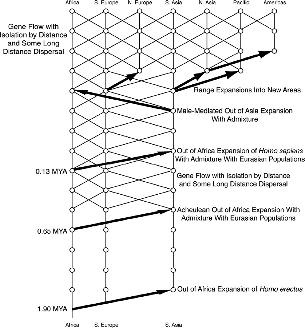
[Consider adding templeton tree image to contrast with the trellis]
The significance of the trellis finding for the question of race is this: the branching hierarchy is real as a description of demographic history. Populations genuinely did separate, pass through bottlenecks, and spread into new territory. That is why Long’s nested subsets model captures the overall topology of human genetic variation so well (R² = 0.94). But the nested subsets model is itself a pure branching tree—and when the hypothesis of treeness has been tested for human populations, it has been rejected in every case [Templeton 2013; Long and Kittles 2003]. Long attributed his model’s imperfect fit to its failure to capture admixture and more complex migration [Long, Li, and Healy 2009], a conclusion confirmed by coalescent simulations showing that the observed global pattern of gene identity variation (gene identity measures genetic similarity between individuals—how it varies across populations reveals the demographic history that shaped current diversity24) fits a model of nested regional bottlenecks overlaid with local gene flow—neither pure isolation by distance nor pure branching alone reproduces the data, but the combination does [Hunley, Healy, and Long 2009, “The Global Pattern of Gene Identity Variation Reveals a History of Long-Range Migrations, Bottlenecks, and Local Mate Exchange: Implications for Biological Race,” American Journal of Physical Anthropology 139:35–46].
The trellis bears on the lineage definition of race in two distinct ways. First, the specific racial categories people have proposed—European, African, Asian—do not correspond to branches of any tree. As the ancient DNA evidence discussed below will show, each of these categories is itself a recent blend of multiple deeply divergent ancestral populations. “Sub-Saharan African” is paraphyletic, as we saw from Long’s analysis. The folk racial categories are historically contingent groupings that do not map onto genetic lineages.
Second, and more fundamentally, even if one abandoned the folk categories and tried to define races using the actual branches of the tree, the lineage definition would still fail. Templeton’s definition requires “barriers to genetic exchange that have persisted for long periods of time” [Templeton 1998]. What his analysis shows is that such barriers never existed: there were no fragmentation events, only range expansions accompanied by gene flow. It is the continuity of gene flow, not its volume, that matters—because what the lineage definition tests for is sustained reproductive isolation, and any ongoing gene flow means the lineage was not independently developing. This is also what prevents saving the lineage definition by retreating to sub-races within the nested hierarchy: at every level of the tree, the same pattern holds. No branch of the human tree ever achieved the sustained independence that the definition requires.
2.2.5 PCA and STRUCTURE
Let’s now return to population structure and the concept of ancestry. Recall that genetic ancestry is measured by genetic similarity (how similar an individual’s genome is to reference populations’ genomes), which means it is quantified by population structure (resulting from non-random mating). One tool for measuring population structure is a Principal Components Analysis (PCA) plot. I will not get into the technical details of what such graphs mean: if the reader has gone through the Genetics 101 sections, they will have enough intuition for responsibly understanding enough of what these graphs portray.
In PCA graphs, genomes are genotyped at many SNPs or other locations of interest (ancestry informative markers). The genotypes are treated as very high dimensional points with an axis/dimension for each locus and then are projected into 2D or 3D. Each dot on a PCA graph represents an individual’s genotype. The axes on a PCA plot are called the “principal axes” and display the axes of greatest variation (recall variation is statistical variation, i.e., a measure of how much the data points vary or are spread out in values): the abstract directions in which the greatest variation lies. See Figure 12 for an illustration of the PCA process. The 99.6-99.9% of the genome that is identical between individuals is not displayed on these graphs because those portions of the genome are not different among individuals. Individuals that lie nearer to each other are more genetically similar to each other; individuals that lie further away are less genetically similar. Since this is a relative comparison, the numbers on the axes are largely meaningless. The percent variation that is sometimes displayed on an axis is not meaningless: it states how much of the total variation is captured going along that axis, e.g., if 75% is displayed on an axis, then the dots along that axis capture 75% of the total variation in the data set. PCA is very sensitive to differences in a data set, and so it is useful in general for observing differences among data points in large data sets.
Under certain assumptions, a PCA graph can be interpreted in terms of ancestry proportions. The distance between individuals on the graph can be related to the generations it takes for the two individuals to have a common ancestor. For individuals of recently-mixed ancestry, they will be projected between individuals of the reference populations from which they were mixed. [[McVean 2009 figure?]]
There are limitations to PCA: the direction of greatest variability is quite abstract, and so the graph says nothing about in what the genetic similarity or differences consist. PCA is also easily influenced by sampling, as seen in Figure 13. Simply by sampling more in one population, the gap increases between that population and the rest, while the rest move more closely together. We again cannot know the true ancestral populations. PCA cannot distinguish between different population histories that produce the graph: an individual falling between other individuals may do so because of recent admixture, or there may be a third population that relates the three individuals together [verify from Gusev figure, which seems to actually be verifying from McVean 2009 and cite him]. And finally, PCA does not tell us anything about the traits (phenotype) of the populations. All it does is show that an individual is more genetically similar to some individuals than to others. As a result, PCA is usually used for exploratory analysis to get a sense of direction for population structure in the data set and then more formal model-fitting analyses are used to test relationships, such as the test for race-like vs nested subset model that we saw.
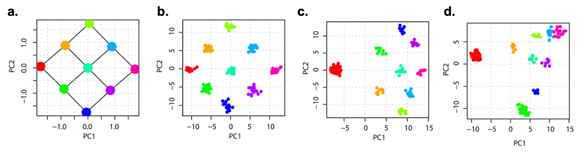
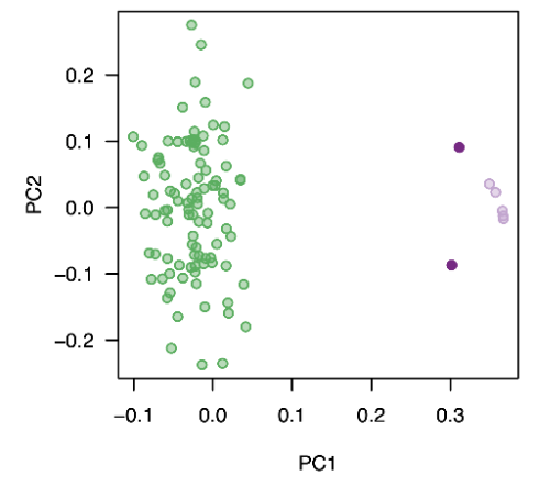
As another example of surprises with PCA visualizations, see this figure from Gusev Figure 14. What are these two clusters? Two different populations? Nope! It is a uniform population and a family, whose parents are from the same uniform population. See Figure 15 for the full figure. Children are so much more closely related to parents that we see a huge gap form between the family and the rest of the population, even though the parents are from that population. If the children are removed and the parents are left behind, we see a random scatter of individuals, as expected for a uniform population. This is a reason why PCA analyses are done on unrelated individuals [support with citation or delete sentence]. What we have seen from both these examples is that gaps on a PCA plot are not necessarily indicative of highly distinct populations, and the gaps and clusterings that appear depend on which individuals are included in the data set.
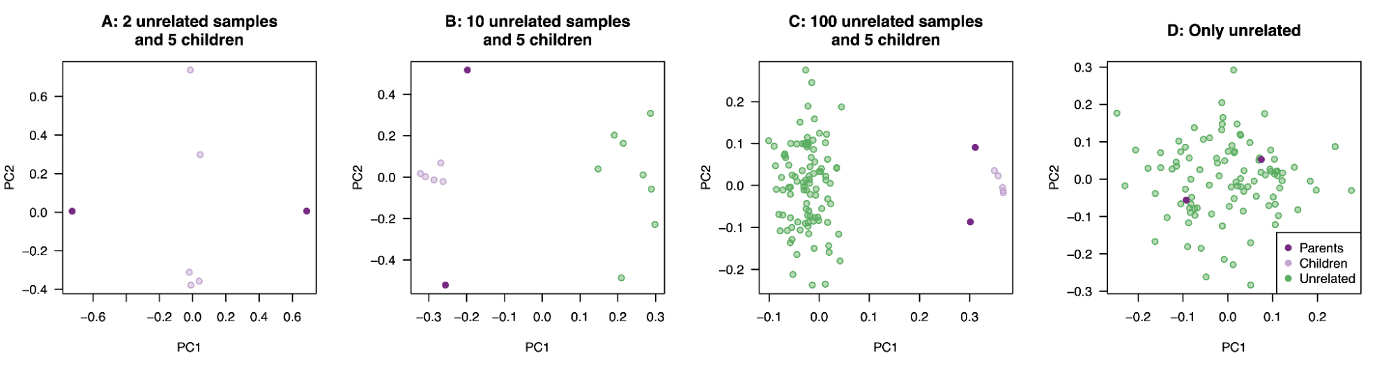
Another way to investigate population structure is through model-based clustering algorithms, the most prominent of which is the STRUCTURE program [Pritchard, Stephens, & Donnelly 2000] and its faster variant ADMIXTURE [Alexander et al. 2009]. These algorithms work differently from PCA, and their differences matter for correctly interpreting the results.
STRUCTURE takes as input the genotype data for a set of individuals and a number K chosen by the analyst. It then assumes that K discrete ancestral populations exist, each in Hardy-Weinberg equilibrium (i.e., each internally randomly mating), and uses probabilistic inference to assign each individual a set of ancestry proportions summing to 1—the estimated fraction of that individual’s genome derived from each of the K ancestral populations. The output is typically displayed as a bar plot: each individual is a vertical bar, and the colored segments of the bar show the estimated proportions from each cluster. Individuals who appear to have ancestry from multiple clusters will have multicolored bars.
Two features of this design are critical for interpreting the results. First, the analyst specifies K before running the algorithm. STRUCTURE does not discover how many groups humans naturally sort into; it is told how many groups to find, and it finds them. If K=2, it divides the world into two groups. If K=5, five. If K=20, twenty. There are statistical methods for comparing different values of K, but none of them identifies a uniquely “correct” K. The most commonly used is the Evanno delta-K method [Evanno et al. 2005], which looks at the rate of change of the model’s log-likelihood as K increases. It does not, however, identify the “true” number of groups. It has a well-documented bias toward selecting the uppermost level of hierarchical structure—the deepest split (smallest K) in the data—rather than the finest resolution. In a review of 1,264 studies using STRUCTURE, Janes et al. (2017) found that delta-K selected K=2 in over half the cases, even when finer subdivisions clearly existed in the data [Janes et al. 2017, [verify journal]]. The alternative approach—examining the log-likelihood directly—is no more decisive: the log-likelihood of the model typically keeps increasing as K rises, because more clusters always fit the data better, just as a higher-degree polynomial always fits data points better. It rarely plateaus clearly at a single value. Cross-validation error (used by the faster ADMIXTURE algorithm [Alexander et al. 2009]) is more principled but still selects which discrete approximation best captures what may be, in reality, a continuous pattern. The developer of STRUCTURE himself, Jonathan Pritchard, recommends in the software’s manual that researchers take a “relatively informal approach” to evaluating K, examining whether the clusters make biological sense and whether individuals are strongly assigned—an acknowledgment that the formal methods alone are not definitive [[verify this is in the STRUCTURE manual]].
In short: statistical methods can tell you which K values fit a particular dataset most stably, but the “best” K depends on the dataset and the sampling scheme. Change the populations sampled and the best K changes with them. No K value reveals the true number of human groups. Moreover, at higher K values, the algorithm increasingly fails to converge on a single solution. Multiple runs with the same K will produce different groupings, because when K exceeds the number of clearly distinguishable groupings in the data or when the boundaries between groups are not sharp (such as when the underlying variation is continuous) there are many equally good ways to partition individuals, and the algorithm has no basis for preferring one over another. We will see shortly what the pattern of human genetic variation actually looks like, and why this matters. This does not mean that such unstable K values are wrong or unlikely: it just means they produce multiple solutions. In fact, sometimes different solutions for a single value of K will have high or low probabilities and may have higher probability than other, more stable values of K!
Second, STRUCTURE assumes that the ancestral populations are discrete. It models the world as a mixture of distinct populations, each with its own allele frequencies. If the underlying genetic variation is actually clinal—shifting gradually across geography with no sharp boundaries—STRUCTURE will still represent it as a mixture of discrete populations. It has no other option; discrete populations are built into the model. This means STRUCTURE will always produce clusters, regardless of whether the actual pattern of variation is clustered or continuous. The clusters are a feature of the model’s assumptions, not necessarily a feature of the data. This is not a flaw in the algorithm—it is a useful tool for summarizing genetic variation—but it means that observing clusters in a STRUCTURE output cannot, by itself, establish that discrete genetic groups exist in reality.
Mathematically, STRUCTURE is closely related to PCA: both methods extract axes of genetic variation and partition individuals along them, and both are sensitive to the same sampling considerations we discussed for PCA. The same caveats apply: clusters in STRUCTURE output do not tell us what the genetic differences consist in, do not tell us whether those differences are in coding or non-coding regions, do not tell us whether the differences produce trait differences between populations, and do not establish that the clusters correspond to races. STRUCTURE detects population structure, and population structure—as we have seen with the Manhattan rats and religious groups—is not the same thing as race.
Having established the picture of what genetic variation actually looks like and investigated PCA and STRUCTURE as tools for investigating population structure, we can now turn directly to the graphs that hereditarians commonly cite and see what they actually show—and what they do not.
2.2.6 Hereditarian PCA and STRUCTURE Claims (Verify)
Hereditarians show graphs like the following. Aside for the “no continuum” labeling, these are real graphs from published scientific literature.
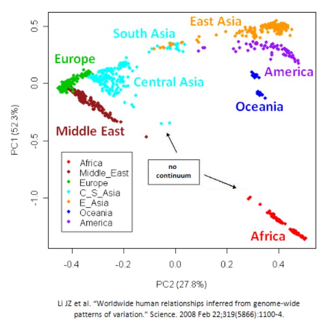
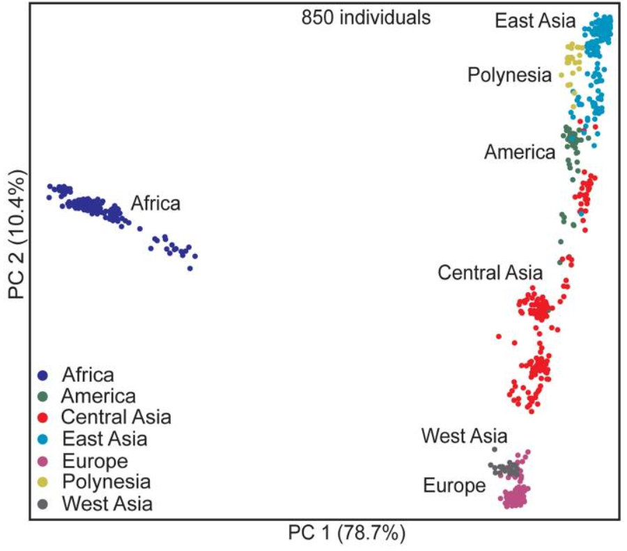
They state that the graphs show the different races genetically cluster in distinct groups with a huge gap between Africans and everyone else. They therefore conclude that the races must be distinct and Africans in particular are very distinct.
However, it should be noted that these graphs—even if they did prove that races were biological—do not say anything about the way in which the races are distinct (Deep or shallow differences? And in what areas are the differences?), nor do they show that the traits of races are immutable. They simply show genetic distinctiveness. Note also that these graphs do not show race but continent—geography, not racial grouping (America means Native American). Genetic ancestry associated with a continent is known as continental ancestry. At best, these graphs show that those with distinct geographical locations can be distinguished genetically: individuals in the data set are more genetically similar to other individuals in the data set who were sampled nearby. Those sampled in regions of Africa cluster with others sampled in similar regions of Africa, and so on.
We can in fact see the locations where these individuals were sampled (Figure 18, Figure 19). Before making further comments on the figures, we should learn about who was actually sampled and who was not. There are three datasets to look at, and each has acknowledged limitations relevant to their interpretation.25
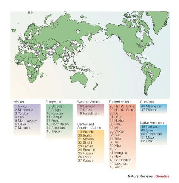
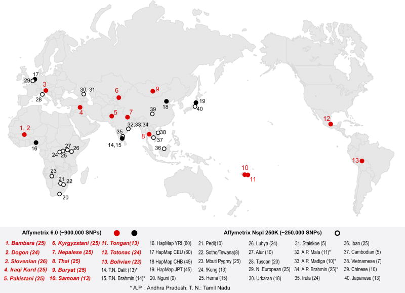
The first dataset is HapMap (International HapMap Consortium 2003, Nature 426:789–96), the reference panel underlying much of the older population-genetics literature and many of the analyses that circulate online. HapMap consisted of just four populations: Yoruba from Ibadan, Nigeria; residents of Utah with northern European ancestry; Han Chinese from Beijing; and Japanese from Tokyo. The Consortium stated that they decided “to include several populations from different ancestral geographic locations to ensure that the HapMap would include most of the common variation” [International HapMap Consortium 2003]—but in the same paragraph acknowledged that “no populations are typical, special or sharply bounded” and that “most common patterns of variation can be found in any population” [International HapMap Consortium 2003]. HapMap Phase II (2007) added more markers but remained the same four populations; HapMap Phase III (2010) expanded to eleven populations but still sampled nothing from North Africa, the Horn of Africa, the Nile Valley, or the Arabian Peninsula. As we will see below, Xing et al. showed that global FST drops substantially when geographically intermediate populations are added to HapMap’s four sites [Xing et al. 2010, Table 2]. Anyone citing analyses built on HapMap reference panels is citing analyses built on four populations selected from opposite ends of the globe, and that selection exaggerates the degree of global differentiation.
The second dataset is the HGDP-CEPH panel, the source of the Li et al. (2008) PCA. The HGDP panel was assembled from cell lines donated by researchers working on human evolution and anthropology. Cavalli-Sforza (2005) explained that all samples come from populations of anthropological interest—those that were in place before the great diasporas of the fifteenth and sixteenth centuries—because only such populations would be useful for disentangling the genetic complexities produced by post-1500 population mixtures [Cavalli-Sforza 2005, Nature Reviews Genetics 6:333–340]. Populations that are recently mixed or geographically intermediate—the ones that would fill in the space between continental clusters on a PCA—were left out by design. Gaps on the sampling map correspond to gaps on the PCA. Li et al. acknowledged that “HGDP-CEPH is not a random sample of the world’s populations” and noted that China and Pakistan are more densely covered than Africa, the Americas, and Oceania [Li et al. 2008]. Consider the imbalance: Africa—the continent with the most genetic diversity—is represented by seven populations in the HGDP panel, while East Asia is represented by roughly eighteen.26 India is not represented at all [Cavalli-Sforza 2005; Xing et al. 2010].
The third dataset is Xing et al. (2010), the source of the second PCA above. The title says it all: “Toward a More Uniform Sampling of Human Genetic Diversity.” Xing et al. set out to fix the sampling limitations of HapMap and the HGDP. Xing et al. added populations from West Africa (Dogon, Bambaran), Central Europe (Slovenian), West Asia (Iraqi Kurd), Central Asia (Kyrgyzstani, Buryat), South and Southeast Asia (Pakistani, Nepalese, Thai), Polynesia (Tongan, Samoan), and the Americas (Bolivian, Totonac). When they added geographically intermediate populations, FST dropped substantially. Their Discussion is blunt: “between-population differences can be seriously exaggerated if human populations are sparsely sampled” and “differentiation among human populations decreases substantially and genetic diversity is distributed in a more clinal pattern when more geographically intermediate populations are sampled” [Xing et al. 2010]. Despite this effort, their sampling still does not cover the Africa-to-Eurasia corridor: there are zero populations from North Africa (other than the Mozabite inherited from HGDP), the Horn of Africa, the Nile Valley, or the Arabian Peninsula. The gap on PC1 in their figure corresponds to the empty band on their sampling map.
What about the huge gap between Africa and the rest? There are two things to notice about this PCA: what the axes tell us about genetic variation and what the gap tells us about who was sampled.
First, the axes. Xing et al. noted that PC1 accounts for 78.7% of total variance and separates African from non-African populations, while PC2 reflects genetic variation within Eurasia [Xing et al. 2010]. That PC1 captures so much of the total variance, and that it orients itself along the Africa-to-non-Africa axis, tells us that the single largest dimension of genetic variation in the data set runs from Africa to everywhere else. This is not a sampling artifact. It is exactly what we would expect from the pattern of genetic variation we have already discussed: non-African populations carry a subset of the genetic variation found within Africa, having passed through a founding bottleneck that produced a systematic offset in allele frequencies. Xing et al. interpreted their data as evidence for a single migration event out of Africa, concluding that the founding population of Eurasia was “relatively large but isolated from Africans for a period of time.” They noted that their results show “the relative homogeneity of European and Asian populations relative to African populations” [Xing et al. 2010].27 This finding—that African populations harbor the greatest genetic diversity and non-African diversity is reduced and derived from an African source—is consistent with the nested subsets pattern we established earlier. The hereditarian, then, is citing a paper whose own authors concluded that non-African populations owe their reduced diversity to descent from an African source population, as if it were evidence for discrete racial categories. It is evidence for the opposite of what the hereditarian claims.2829
But what about the gap itself—the empty space along PC1 between the African and non-African clusters? Here the answer is different. The gap is not what tells us about the magnitude of genetic variation; PC1’s variance percentage does that regardless of whether there is a gap. What the gap tells us is that no populations in this particular data set have intermediate values along PC1. And the reason for that is straightforward: Xing et al. did not sample any populations from the Africa-Eurasia corridor. Their paper, titled “Toward a More Uniform Sampling of Human Genetic Diversity,” added populations in West Africa (Dogon, Bambaran), Central Asia (Kyrgyzstani, Buryat), Polynesia (Tongan, Samoan), and the Americas (Bolivian, Totonac)—but zero populations from North Africa, the Horn of Africa (Ethiopians, Somalis, Eritreans), the Nile Valley (Nubians, Sudanese Arabs), or the Arabian Peninsula. These are precisely the populations whose geographic position and known genetic history would place them in the gap between the African and Eurasian clusters. And when other studies do sample these populations, that is exactly where they appear:
- Kidd et al. (2019), using 76 reference populations with North African and Southwest Asian coverage, found that PC1 “organizes the data from West Africa at one extreme to Northern Europe at the other extreme” with “a clear clinal organization of the North African to Southwest Asian to European populations”—continuity along the very axis where the gap appears in HGDP-based PCAs [Kidd et al. 2019, European Journal of Human Genetics] [verify].
- Henn et al. (2012) genotyped seven North African populations spanning from Egypt to Morocco at 730,000 SNPs and found that these populations occupy PCA space between sub-Saharan Africa and Europe/Middle East [Henn et al. 2012, PLoS Genetics] [verify].
- Hollfelder et al. (2017) genotyped 221 individuals from 18 populations in Sudan and South Sudan and found a gradient from near-sub-Saharan to near-Eurasian positions in PCA space. Northeastern Sudanese populations (Nubians, Arab groups, Beja) carry 40–48% Eurasian ancestry, while southern Nilotic populations show little or no Eurasian admixture—creating a continuous grading across the gap [Hollfelder et al. 2017, PLoS Genetics] [verify].
- Serra-Vidal et al. (2024), analyzing 364 whole genomes at 1.58 million SNPs, found “North African individuals clustered together in-between sub-Saharan African and Eurasian populations” on PC1-PC2, with East North Africans closer to Middle Easterners and West North Africans further away—a gradient within the intermediate space itself [Serra-Vidal et al. 2024, Genome Biology] [verify].
The gap in Xing’s PCA is not a gap in human populations. It is a gap in Xing’s sampling. The populations that would fill it exist, and when sampled, they do fill it.
A critical point follows from this. Even with the gap filled in, the fundamental asymmetry in the PCA persists—and this asymmetry is evidence for the nested subsets model, not for discrete races. African populations still span the greatest range along PC1, the axis of greatest variation, because Africa holds the most genetic diversity. Non-African populations differentiate more along PC2 and subsequent components, which capture far less of the total variance. Filling in the gap removes the visual impression of two discrete clusters separated by empty space; it does not remove the fact that the largest dimension of human genetic variation runs from Africa outward—exactly what nested subsets predicts. What the hereditarian needs from these PCA graphs is the discreteness—the empty gap that could justify drawing a boundary between races. That is the part that is a sampling artifact. What survives with better sampling is a continuous gradient of genetic variation in which Africa occupies the broadest range—the nested subsets prediction.
To put it another way: the founding event left a real allele-frequency offset on PC1 between African and non-African populations. That offset is biological, and it is what makes PC1 the dominant axis. Whether that offset appears as a gap with empty space or as a populated gradient with intermediate populations is a separate question, answered by who was sampled. The hereditarian reading of these graphs conflates allele-frequency differentiation—which is real—with population discreteness—which is an artifact of who got sampled.
There is a deeper point here about what the gap consists in. Recall that PCA axes display the directions of greatest genetic variation. The variants that contribute most to the separation between populations on a PCA plot—those with the highest “loadings” on PC1 and PC2—are the variants with the largest allele-frequency differences between the sampled populations. But a large allele-frequency difference tells you nothing about what that variant does. The variant might affect a trait; it might sit in a regulatory region that influences gene expression; or it might have no biological function at all. PCA does not distinguish between these possibilities. It measures genetic distinctiveness—full stop. Whether that distinctiveness translates into differences in traits like cognitive ability is a separate question entirely, and it requires separate evidence. We take up that question directly in the section on quantifying population differences.
Aside from PCA, hereditarians often like to point to algorithms like STRUCTURE that they claim show five races corresponding to continents [[show Rosenberg figure]].
Look at this figure. The hereditarian sees five clean blocks of color that look like five distinct groups. Let us examine what is actually being shown and what it does and does not establish.
First, recall what we discussed about how STRUCTURE works: the user specifies K, and the algorithm sorts individuals into that many clusters, assigning individuals to multiple clusters if necessary. At K=2, global human variation partitions into Africa vs. non-Africa. At K=5, roughly continental groupings appear. At K=6, the additional cluster is not another continent but the Kalash—a small, geographically isolated population from northwest Pakistan that has accumulated distinctive allele frequencies through genetic drift. This is not a failure of the algorithm; STRUCTURE is doing exactly what it does, detecting population structure at progressively finer scales. But it reveals what the algorithm is actually finding: a hierarchy of genetic distinctiveness driven by geographic barriers and drift, not a fixed set of races.
Rosenberg’s ten runs at each K produced nearly identical results at K=2 through K=5 (pairwise similarity coefficients above 0.97). At K=6, one of ten runs produced a different sixth cluster—splitting off the Karitiana, an indigenous South American group, instead of the Kalash [Rosenberg et al. 2002]. Beyond K=6, runs became increasingly inconsistent, producing different groupings depending on the random seed. This instability reflects the fact that the HGDP panel, with its sparse and geographically separated sampling, did not contain enough intermediate populations to support stable finer-resolution partitions. At these higher values of K, the algorithm could no longer even agree with itself about how to partition the genetic variation. As we will see, denser sampling does not rescue five races; it multiplies the stable clusters far beyond what any racial scheme can accommodate.
The stability of the solution does not privilege K=5 over K=2, K=3, or K=4—all were equally stable. Indeed, the most commonly used statistical method for selecting K, the Evanno delta-K method, has a well-documented bias toward selecting K=2 [Janes et al. 2017; Waples & Gaggiotti 2006]—meaning that if the hereditarian wishes to take K-selection methods seriously, the statistically favored number of human groups is two, not five, and in that grouping Europeans, East Asians, Native Americans, and Melanesians all fall into the same cluster. That is not a racial scheme anyone has ever proposed. The appearance of “five races = five continental clusters” is an artifact of the analyst’s choice to display K=5—conveniently matching the classical continental races. The algorithm did not discover five races; it was instructed to find five groups, and it dutifully did so. Authors of papers typically post results for a range of K values precisely to give a sense of how human genetic variation distributes at multiple resolutions, not to identify the “correct” number of races. When the hereditarian selects K=5 as the correct value it is simply because it matches the racial scheme they already had in mind.
Second, the visual sharpness of the color boundaries in this figure is partly a consequence of how it is drawn. The individuals in the plot are sorted by their pre-assigned population label, and those populations are then grouped by continent. All the African populations are placed together, then all the European populations, then all the East Asian populations, and so on. This sorting is done before the figure is drawn—it is a decision made by the person constructing the graphic, not a result produced by the algorithm. The sharp visual transitions between color blocks correspond to the places where the analyst drew the continental boundaries on the x-axis. Where populations from geographically intermediate regions are included (Central Asia, the Middle East, North Africa), the bars are typically multicolored—showing mixed ancestry from neighboring clusters—but these populations are few in the HGDP panel, and the sorting places them at the edges of their continental group where they are easy to overlook.
Third, the sampling matters. The Rosenberg (2002) STRUCTURE analysis used the HGDP panel, whose sampling limitations we described above: populations assembled from geographically separated groups of anthropological interest, with the geographically intermediate regions left largely unsampled (and combined with the four HapMap populations, which were selected from opposite ends of the globe [International HapMap Consortium 2003 https://www.nature.com/articles/nature02168]). Serre and Pääbo (2004, Genome Research) argued that the apparent clusters were partly a consequence of this uneven sampling and showed that with more geographically uniform sampling, the degree of clustering diminished. Rosenberg et al. (2005, PLoS Genetics) responded by expanding from 377 to 993 markers and systematically testing the influence of study design on clustering. They showed that with enough markers, some clustering is robust—I will grant this. Continental-scale clusters survive improved sampling when sufficient genetic markers are used, and there is no point in denying it. But they also conceded that the apparent visual discreteness of these plots is shaped by where samples were drawn. Gaps on these plots are, in substantial part, gaps on the sampling map. [[verify Serre & Pääbo 2004 and Rosenberg 2005 details]] There is a deeper reason for this than uneven coverage. STRUCTURE assumes discrete ancestral populations and fits the data to that model—and it has been shown that STRUCTURE generates well-differentiated apparent clusters as a mathematical artifact of coarse geographic sampling from any species characterized by isolation by distance [Frantz et al. 2009, Journal of Applied Ecology; Safner et al. 2011, International Journal of Molecular Sciences]. The algorithm imposes discrete structure on what is in reality continuous variation. When Behar et al. (2010) sampled Old World populations more finely and ran STRUCTURE, the result was telling: most individuals showed significant genetic input from two or more clusters, and clean group membership dissolved [Templeton 2013]. We will return to what STRUCTURE shows with modern data and better sampling shortly. For now, the key point: STRUCTURE does not show race is real, and even if it did, it would not state whether the genetic distinguishability is due to traits that are immutable, what traits they are, or even whether the distinguishability results in trait differences at all (more on this when we talk about quantifying differences between populations).
2.2.7 PCA, STRUCTURE clusters, Population Structure, and Continuous Ancestry - AI gen
Recall that the PCA graphs we have investigated use small, geographically uneven samples, each with acknowledged limitations. HapMap used four populations from opposite ends of the globe to capture as much common variation as possible. The HGDP excluded post-1500 admixed populations by design. Even Xing et al.’s explicit effort at more uniform sampling left the Africa-to-Eurasia corridor empty. What happens when we collect samples from different races and plot their ancestry using PCA, and what happens when we have better and less limited sampling? With modern data from large biobanks (thousands to hundreds of thousands of samples) and genome sequencing with better sampling, let us now look at self-identified race (SIRE; the race that someone checks off on a box in a questionnaire) and see what relationships we find.
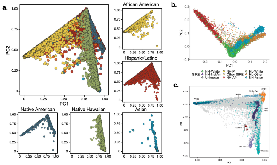
[Gusev: “(a) The PAGE cohort of primarily non-white participants separated by self-reported race shows continuous genetic ancestry in all groups [Figure from (Wojcik et al. 2019)]. (b) The ATLAS cohort from the UCLA health system, color-coded by race recorded in the electronic medical record [Figure from (R. Johnson et al. 2022)]. (c) The BioMe biobank collected in New York City (gray points) overlapped with data from HapMap/1000 Genomes reference populations (color coded) [Figure from (Lewis et al. 2022)].” NH = Non-Hispanic; HL = Hispanic Latino]
First, a brief note on what these graphs depict in terms of ancestry. The axes of these graphs are made using reference populations, which usually appear at the corners of these triangular shapes. For recently admixed individuals, they will appear approximately where they should appear even if the reference populations are missing. So figure (a) for example, although it is missing a sample of white SIRE, is showing what it would show even if whites were there. This is confirmed by comparing it with figure (b).
Now, let’s look at these graphs. We see that ancestry is continuous: there is a gradient of ancestry between reference populations at the corners of the triangles. Looking at figure (a), African Americans span a large space between the African corner of the graph and European corner of the graph, and there are individuals making their way to the Asian corner of the graph. In figure b, we see the gradient of African Americans again, and we see non-Hispanic whites overlapping with the African American continuum.
What we see here is what is seen in the general case with modern data. There are no clusters: there is just one big cluster with a continuum of ancestry. There is no way to non-arbitrarily divide the ancestry space. Furthermore, going the other direction, race does not make a clean division in the ancestry space: there is lots of overlap. There is an important distinction between race and ancestry.
At this point, hereditarians shift the goal posts (remember how they say “no continuum” on a previous graph?). They counter with 1) there are fewer individuals of mixed ancestry, so the graphs are misleading, and 2) those of the same race do cluster near each other.
In answer to 1), the number of individuals sitting near a mode does not determine whether a biological kind exists. Icelanders are not less of a population because they are few; a billion-strong European mode is not more of a race because it is large. If density peaks constitute races, then race-hood depends on census size: the wrong kind of fact for a biological kind. Headcount can be evidence of structured mating; it cannot be constitutive of kind-hood. Moreover, the sharpness of peaks on biobank PCA plots is partly an artifact of sampling: a biobank with 500,000 participants from one region and 5,000 from another will show the first as a mountain and the second as a speck, regardless of biology. The ancestry continuum is seen whenever any PCA or other clustering tool is used, whatever the number density of individuals might be, so long as the sampling is done well. The number density argument receives a fuller treatment below.
In answer to 2), yes, individuals of the same self-identified race do tend to cluster near each other—because race correlates with geography and ancestry, and geography creates population structure. But clustering arising from population structure does not establish that the correlated category is biologically real. Recall that uptown and downtown Manhattan rats cluster genetically too; they are not separate races of rats. We will see more plots that support this in a moment, and these objections will be addressed more fully when we consider attempts to equate race and ancestry.
The point generalizes beyond geography. PCA can distinguish any non-randomly-mating group, including groups that no one would call separate races. Haber et al. (2013, PLOS Genetics) analyzed Lebanese individuals from different religious communities—Maronite Christians, Druze, Shia Muslims, and Sunni Muslims—and found that PCA and STRUCTURE could distinguish them genetically [Haber et al. 2013, “Genome-Wide Diversity in the Levant Reveals Recent Structuring by Culture,” PLOS Genetics 9(2): e1003316; verify]. These are all people of the same nationality, the same geographic region, and the same “race” under every racial classification scheme that has ever existed. They are genetically distinguishable because religious endogamy—marrying within one’s religious community—has created population structure over centuries. PCA detects that structure, just as it detects the structure between Manhattan rat populations or between neighborhoods in Chinese cities. Population structure is ubiquitous, and PCA will find it wherever non-random mating exists. The hereditarian who argues from PCA clustering to biological race must explain why Lebanese Maronites and Lebanese Druze are not separate races—or accept that genetic distinguishability, by itself, does not establish racial categories.
What about STRUCTURE with modern data and better sampling? The results are instructive, and they do not help the hereditarian.
I will grant what should be granted: continental-scale clusters are robust. Rosenberg et al. (2005) showed this, and more recent analyses with larger marker panels and more individuals confirm it. If you run STRUCTURE on a global dataset with enough markers, you will find clusters that correspond to major geographic regions. This is not in dispute.
But recall what STRUCTURE actually does: it assumes K discrete ancestral populations and fits the data to that model. It will always find clusters because clusters are built into the model. The question is not whether clusters appear, but what they mean and whether they map onto racial categories. Here the modern data is devastating to the hereditarian position.
The most important development is what happens when Africa is sampled properly. The older analyses that hereditarians cite—Rosenberg (2002), Li et al. (2008)—used the HGDP panel, which included only a handful of African populations. Africa, the most genetically diverse continent, was represented by a few geographically scattered groups. When Tishkoff et al. (2009, Science) analyzed 121 African populations with 1,327 markers, they identified 14 ancestral population clusters within Africa alone [Tishkoff et al. 2009, “The Genetic Structure and History of Africans and African Americans”]. The entire continent that hereditarians lump together as one “race” contains as many or more genetically distinguishable clusters as the rest of the world combined.
[Tishkoff 2009 figure]
With denser, more geographically representative sampling, the instability that plagued Rosenberg’s analysis at K=6 largely disappears—but what replaces it is not fewer, cleaner racial clusters. It is more clusters, reflecting the finer-grained population structure that sparse sampling missed. The algorithm was splitting off drift outliers like the Kalash at K=6 because the HGDP panel lacked the intermediate populations needed to support meaningful higher-K solutions. Give the algorithm those populations, and it finds them—fourteen in Africa alone.
This point is made even more vividly by an infographic published in Nature [Carlson et al. [verify exact citation—this appears to be a Nature commentary or infographic piece, possibly with Sohini Ramachandran as co-author; the escholarship link is https://escholarship.org/uc/item/7gg7r4fp]] that directly compares what STRUCTURE shows with sparse versus dense African sampling. [Insert Carlson/Ramachandran Nature figure here.] In the left panel, with African populations making up only 13.5% of the sample (mirroring the HGDP-era analyses), the familiar picture of a few seemingly clean continental clusters appears. In the right panel, with African representation boosted to 85% of sampled populations, Africa fractures into multiple distinct clusters—Southern Africa, Western Africa, the African Great Lakes region, the Horn of Africa—while the genetic differentiation within Africa is shown to be comparable in magnitude to the differentiation between the non-African continental groups. The article further notes that the version of this figure with sparse African sampling was reproduced in the manifesto of the gunman who killed ten Black people in Buffalo, New York, in May 2022. The “five races” picture was an artifact of undersampling the most genetically diverse continent on earth—and it is being weaponized.
Similarly, Henn et al. (2011, PNAS) showed that African hunter-gatherer populations (the Hadza, Sandawe, and ≠Khomani Bushmen) retain highly differentiated ancestry components not found in other African populations, with distinct clusters emerging at K=4 and K=8 [Henn et al. 2011, “Hunter-gatherer genomic diversity suggests a southern African origin for modern humans”]. The more carefully you sample Africa, the more structure you find. None of it maps onto “Black” as a meaningful genetic unit.
The hereditarian might respond: “Fine—those are sub-races of the main African race, and we still have the continental races above them.” This goalpost shift receives a fuller answer below when we discuss race as the largest global population structure. Briefly: if 14 African clusters are sub-races, and fineSTRUCTURE finds 17 clusters in Britain alone [Leslie et al. 2015], and Sakaue et al. (2020) finds 11 in Japan, you rapidly reach hundreds of “sub-races” with no principled stopping point. “Race” collapses into “population at some resolution,” which is a concept geneticists already have without racial baggage.
What does the author of the very paper hereditarians cite most frequently say about the pattern of genetic variation his own data reveals? In Rosenberg et al. (2005), titled “Clines, Clusters, and the Effect of Study Design on the Inference of Human Population Structure,” the authors showed that allele frequency differences generally increase gradually with geographic distance. The clusters, they found, arise from “small discontinuous jumps in genetic distance for most population pairs on opposite sides of geographic barriers”—oceans, the Himalayas, the Sahara [Rosenberg et al. 2005]. Rosenberg further stated that “genetic differences among human populations derive mainly from gradations in allele frequencies rather than from distinctive ‘diagnostic’ genotypes” and explicitly cautioned that these findings “should not be taken as evidence of our support of any particular concept of biological race” [[verify exact location of these quotes—they may be from Rosenberg et al. 2002 rather than 2005]].
In other words, the data shows genetic variation that is predominantly gradual—shifting smoothly with geographic distance—with small discontinuities (just 1-2% of the microsatellite variation) where geographic barriers like oceans and mountain ranges have historically limited migration. The clusters are real, but they are products of geography, not of racial biology. They track barriers to human movement, not natural kinds. And even within the clusters, variation is itself continuously structured along geographic gradients, as we are about to see.
We see continuous ancestry when looking across races, and the same pattern holds within them. PCA detects continuous population structure at every scale it is applied to, even within supposedly homogeneous racial groups, provided there are enough samples.
Two large-scale studies of individuals all classified as “White” illustrate this. Galinsky et al. (2016) applied PCA to roughly 55,000 individuals from the GERA cohort in Northern California, restricting the sample to those with minimal genetic similarity to non-European reference populations—filtering out, in other words, everyone who might introduce cross-continental variation. Even after this filtering, the remaining “White” individuals showed continuous clines of ancestry reflecting European geography: North/South and East/West gradients, not discrete clusters. When the GERA data was overlaid with samples from specific European countries, the American individuals fell along the same geographic gradients as their European counterparts. Agrawal et al. (2020) went further still, applying PCA to approximately 280,000 “White British” individuals in the UK Biobank—all self-identified as the same race and filtered for genetic similarity to European references. The leading principal components correlated with geography within Britain itself: north versus south, east versus west. Population structure appeared at a scale far below anything anyone would call a racial boundary. Gusev summarizes both studies:
“[F]ine scale population structure is clearly observed even when restricting to seemingly racially”homogenous” populations. Two large scale studies of “White” individuals in the US and UK are highlighted in the figure below. (Galinsky et al. 2016) applied PCA to ~55k individuals from the GERA cohort (primarily collected in Northern California) after restricting to those with minimal genetic similarity with non-European reference populations. This analysis revealed the expected clines of population structure reflecting recent geography. When combined with individuals sampled from specific regions of Europe, the leading PCs showed correlation with North/South and East/West European countries, with substantial continuous ancestry between these groups (see panel a below). (Agrawal et al. 2020) applied PCA to ~280k unrelated “White British” individuals (identified based on self-reported race and genetic similarity with European reference populations) with known geographic birth coordinates. The leading PCs showed substantial structure and correlation with geography of the United Kingdom, including multiple North/South and East/West clines (see panel b below).” [Gusev]
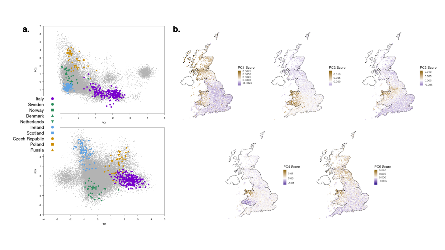
[image of GERA cohort] (a) PCA in the US GERA cohort overlaid with populations sampled from parts of Europe (color coded) [Figure from (Galinsky et al. 2016)]. (b) PCA in the UK Biobank plotted along geographic birth coordinates [Figure from (Agrawal et al. 2020)]. [Gusev]
We see then continuous ancestry among socially-defined races. We see largely continuous ancestry with structure within a socially defined race in the UK that correlates with geography. PCA continues to show the same patterns to the smallest of scales, as seen in the next figures.
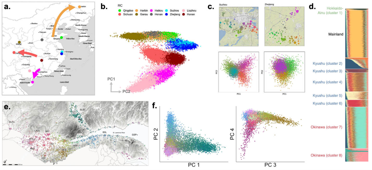
[Continuous ancestry in China] (a, b, c) Geographic sampling, leading Principal Components, and fine-scale Principal Components within individual neighborhoods for individuals in the China Kadoorie biobank [Figures from (Walters et al. 2023)]. (d) STRUCTURE analysis revealing 11 clusters in the Biobank Japan [Figure from (Sakaue et al. 2020)]. (e, f) Geographic sampling and leading Principal Components for individuals from Quebec, Canada [Figures from (Anderson-Trocmé et al. 2023)] [Gusev]
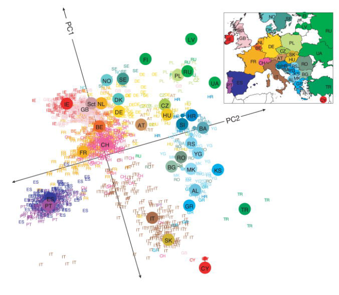
[Genes mirror geography within Europe] “Genes mirror geography within Europe (2008). The plot shows the PCA projection of 1387 European individuals. Each two-letter code shows the projection of a single individual, and the circled letters show the average projections of individuals from the corresponding country. The map in the upper-right gives the two-letter country codes. After slightly rotating the PCA axes, the PCA projection reflects the geographic positions of countries to a remarkable degree, with only minor distortions.” [Pritchard]
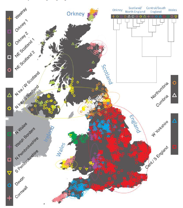
[fineSTRUCTURE in Britain and Northern Ireland] “Fine structure of Britain and Northern Ireland. 2, 039 individuals were clustered into 17 groups using fineSTRUCTURE. Each data point indicates the geographic sampling location, and the symbols indicate the assigned cluster. The bars at left and right indicate labels assigned to each based on their geographic distribution.” [Pritchard]
“In short, continuous ancestry clines are observed within racial groups (Asia), within”sub-racial” groups (China/Japan), within “sub-sub-racial” groups (cities in China), within “sub-sub-sub-racial” groups (neighborhoods in cities in China) and so on.”[Gusev]
We see then that a race model fits the pattern and complexity of genetic variation poorly. Race is discrete, genetic variation is continuous, and it is largely continuous at all scales and levels. Geography correlates with clusters but is not biological; the correlation of race with clusters does not necessarily indicate that it is biological either. In addition, we still have the problem of race not fitting the nested subset model. The only way out is for the race scientist to redefine race so as to match the data—a category that is continuous and cuts across the social races that we have defined.
[[This data is all on modern humans: do we have any idea of population structure in the past? We do indeed, and we find similar patterns of continuous ancestry [[find citation]]. Moreover, we find that the ancestral groupings fall along different geographical lines, i.e., any populations today are not the same as populations in the past, and there are no pure “races.” European ancestry is in fact seen to be a combination of three main contributions [[citation and give what they are from Pritchard; show graph too; maybe give Reich quotation]]. We see from the data that historically, mixture of ancestry is common and the norm!]][marked for deletion; it is now expanded into its own ancient dna section]
2.2.8 Ancient DNA — No Pure Races, Mixing Is Normal - AI gen
This data is all on modern humans: do we have any idea of population structure in the past? We do. Over the past decade, the sequencing of ancient DNA from human remains has opened a window into past population structure that modern data alone cannot provide. And the picture it reveals directly confirms the trellis pattern — branching and remixing, not clean separation — that we described in the nested subsets section above. It is not a picture of stable racial groupings maintained over time, but of constant movement, mixture, and replacement, such that the populations we see today are not the same populations that existed in the past, and the ancestral groupings fall along different geographical lines than modern ones.
Pickrell and Reich (2014) surveyed the ancient DNA evidence and concluded that simple models of populations splitting off and staying put are “no longer supported by genetic data.” They write: “It is now clear that the data contradict any model in which the genetic structure of the world today is approximately the same as it was immediately following the [initial] expansion. Instead, the last 50,000 years of human history have witnessed major upheavals, such that much of the geographic information about the first human migrations has been overwritten by subsequent population movements” [Pickrell and Reich 2014].30 In the decade since, this conclusion has only become more firmly supported.
[Figure: Rough timeline of major migrations and admixtures. Figure from Pickrell and Reich 2014; reproduced by Gusev section 9.10]
The most concrete example comes from Europe. Ancient DNA has revealed that present-day Europeans are not descended from a single ancestral population but are a mixture of at least three deeply divergent groups: (1) Western Hunter-Gatherers (WHG), who inhabited Europe during the Mesolithic period; (2) Early European Farmers (EEF), who migrated into Europe from Anatolia (modern Turkey) and largely replaced the hunter-gatherers; and (3) Steppe Pastoralists related to the Yamnaya culture, who expanded from the Pontic-Caspian steppe during the Bronze Age [Lazaridis et al. 2014, Nature; Haak et al. 2015, Nature; Reich, Who We Are and How We Got Here, 2018]. Every modern European carries ancestry from all three groups, in varying proportions across the continent — more farmer ancestry in the south, more steppe ancestry in the north. There is no “original” European: the category is itself a product of mixture.
[Figure: European ancestry proportions showing the three-way mixture across the continent. Figure from Lazaridis et al. 2014 or Pritchard [verify which graph to use]]
The speed of this mixing could be dramatic. Olalde et al. (2018, Nature) showed that roughly 90% of the ancestry in Britain was replaced within a matter of centuries when the Bell Beaker cultural complex arrived around 4,500 years ago. Before the Beaker migration, the inhabitants of Britain were primarily descended from Neolithic farmers. Afterward, steppe-related ancestry dominated the population. This was not a slow blending over millennia; it was a rapid and near-total genetic transformation [Olalde et al. 2018; Gusev section 9.10].
[Figure: Rapid replacement of >90% of Neolithic British ancestry through expansion of the Beaker complex ~4,500 years ago. Figure from Olalde et al. 2018; reproduced by Gusev section 9.10]
Nor was Europe unique. In the Americas, contemporary Latin American populations show substantial fractions of European, Native American, and African ancestry in varying proportions. STRUCTURE analysis estimates the Native American similarity of Mexican, Colombian, and Puerto Rican individuals at just 48%, 25%, and 13% respectively [Gravel et al. 2013]. And those Native American reference populations themselves trace ancestry to groups that mixed across the Pacific: Ioannidis et al. (2020) identified genetic sharing between Polynesian and Native American samples consistent with contact across the largest ocean on Earth, before any modern transportation existed. In Bronze Age Europe, Antonio et al. (2024) found that at least 7% of ancient individuals at any given site were ancestry outliers, showing significant ancestry from a distant region, some spanning major geographic barriers. Ancient people traveled for work, trade, and resettlement just as people do today [Antonio et al. 2024; Gusev section 9.10].
How could so much gene flow have happened before modern travel? Two mechanisms, both well-established. The first is simply migration: people moved, sometimes very far, as the Polynesian and Bronze Age outlier data show. The second is subtler and arguably more important for the global pattern: even without anyone traveling far, genetic variants propagate across a landscape through local mating with neighbors. Each generation, individuals mate primarily with those nearby, and their offspring carry alleles from both parents into the next generation’s local mating pool. Over many generations, an allele can spread across a continent through this process alone like a wave travelling through water. Mathematically, it behaves identically to the diffusion of heat through a solid, where no single particle travels far but the temperature change propagates steadily. This is known as “isolation by distance” in population genetics, first formalized by Sewall Wright [Wright 1943, Genetics]. The stepping-stone model [Kimura and Weiss 1964] makes this concrete: an allele moves from population A to neighboring B, then B to C, then C to D, without any individual traveling more than a short distance. This process is why genes mirror geography in PCA plots [Novembre and Stephens 2008, Nature Genetics]. The clinal gradients we observe in PCA plots are the natural outcome of local mating propagating genetic variation across space, combined with long-distance migration.
The combination of these two mechanisms — local diffusion and long-range migration — means that gene flow across continents is essentially inevitable over any substantial time period. The ancient DNA record confirms it happened pervasively.
As David Reich, the leading figure in ancient DNA research, has written: “The genome revolution has taught us that great mixtures of highly divergent populations have occurred repeatedly. Instead of a tree, a better metaphor may be a trellis, branching and remixing far back into the past” [Reich, Who We Are and How We Got Here, 2018]. There was, as he puts it, “never a single trunk population in the human past. It has been mixtures all the way down.” The ancient DNA evidence has been so decisive on this point that Reich concludes: “Mixture is fundamental to who we are, and we need to embrace it, not deny that it occurred” [Reich 2018; quoted in Gusev section 9.10].31
This is the same trellis that Templeton inferred from modern DNA alone, before the ancient DNA revolution made direct confirmation possible. As we saw in the nested subsets section, his multi-locus analysis of 25 genomic regions found no statistically significant population fragmentations in human history: the major demographic events were range expansions with admixture, not clean splits followed by isolation [Templeton 2005, 2013]. At the time, this was a minority position — most geneticists reading the data favored models in which expanding populations completely replaced existing ones with no genetic exchange, and some formal analyses assigned near-zero probability to any model involving even slight admixture [Fagundes et al. 2007; Templeton 2013]. Templeton’s nested clade analysis was the only phylogeographic method to reject the no-admixture null hypothesis with strong statistical significance [Templeton 2002, 2005]. When it became possible to sequence DNA directly from ancient remains, the admixture he had predicted was confirmed: both Neanderthal and Denisovan genomes showed low but unambiguous levels of genetic exchange with expanding modern human populations [Green et al. 2010; Reich et al. 2010].32 The pervasive mixture the ancient DNA revolution has since revealed across modern human populations — Europeans as a three-way blend, near-total population turnovers in Britain, ancestry outliers spanning continents in the Bronze Age — is what the trellis predicted. The trellis is not a niche result from one statistical method; it is the consensus picture of human population history, confirmed independently by ancient DNA, by the isolation-by-distance pattern in modern genetic data [Ramachandran et al. 2005], and by the formal rejection of treeness in every dataset where it has been tested [Long and Kittles 2003; Templeton 2013].
For readers who hold to a biblical timeline, this evidence is worth pausing over. The evolutionary account holds that these mixing events unfolded over tens of thousands of years. On a post-Flood timeline of roughly four millennia, all of this occurred even faster. Mixing was not a slow background process but the dominant feature of human population history from the start. There were no “pure races” in the past to be preserved or diluted. This is consistent with what Scripture shows: the Table of Nations (Genesis 10) describes a moment of dispersal, not permanent sealed-off groupings. Moses married a Cushite (Numbers 12:1). Ruth was a Moabitess. Rahab was a Canaanite. Nations have always moved and mingled, and the genetics confirms it.
2.3 Attempts to equate race and ancestry
Sometimes, in the face of the data, hereditarians attempt to redefine race in a way that equates to genetic ancestry. The problems with that are many. We cannot know true genetic ancestors: we only measure genetic similarity. Hence, we cannot know true race if it is equated with ancestry. Moreover, the continuous ancestry space makes it arbitrary where to make the cuts to define racial groupings. These groupings are important: on this basis, stereotypes about groups are made and potentially, discrimination, segregation, and forbidding of marriages as unwise or unlawful. The stakes are too high to define race arbitrarily. Also, ancestry cuts across racial boundaries and would separate into groups those who are supposedly in one race if similarity in ancestry was used to define race, making a racial distinction based on ancestry unlike racial schemes today.
However, the real problem with equating race to ancestry is not lack of identifiability in the given data or lack of accurately mapping to true ancestry. The real issue is what has been noted above: race and ancestry are truly different concepts, and ancestry does not correspond to any of our racial groups. Racial schemes—however they are defined—are discrete, not continuous. Race lumps people together who are greatly genetically diverse (all the great diversity of Africa or SubSaharan Africa is lumped into one “black” race!) and places into different groups those who are greatly genetically similar. Race is inherited socially and is determined socially; ancestry is inherited biologically and is independent of definition in the sense that the genetics blocks are what they are and do what they do, regardless of how we label them. race is an absolute concept: into what category does a person fit; ancestry is a relative concept—how genetically similar are individuals to each other. Race does not obey the nested subsets model that the genetic variation data presents; ancestry fits it just fine. Being a relative concept, ancestry inherently has a sense of scale: we can look at global scales or at the scales of families; race concepts do not always have a sense of scale (sometimes they do when they think in terms of sub-races and sub-sub-races). Race and ancestry also differ in how they behave across generations. Racial categories are fixed social bins: “Black,” “White,” “Asian” persist as labels even as the people assigned to them change. Ancestry, by contrast, is reshuffled every generation. Each child inherits a new recombinant mosaic of genomic segments from both parents, occupying a point in ancestry space that has never existed before. The ancestry distribution of a population is therefore continuously in flux—not because the categories are changing, but because the underlying genetic reality is being remixed with each conception. Meanwhile, for a single individual, race is a less stable category, since the classification bins or how to classify into the bins can change.
Race and ancestry also differ in how they behave across time. Racial categories are discrete social bins that are treated as if they were permanent fixtures, even as the people assigned to them change. But the bins themselves are not truly stable, and different countries carve the same ancestry space into entirely different racial schemes, as we have seen. For any single individual, race is likewise unstable: a person’s racial classification can change through reclassification, movement to a country with a different classification, or shifting social definitions, without any change in their biology. Even when a racial label does persist, the biology underneath it shifts: the label “Black” has been in continuous use in America for centuries, but the average African American today carries substantially more European ancestry than those who bore the same label two hundred years ago. Ancestry is the reverse on both counts. At the population level, the ancestry distribution is continuously in flux: each child inherits a new recombinant mosaic of genomic segments from both parents, occupying a point in ancestry space that has never existed before, and the distribution is remixed with each generation. But for any single individual, genetic ancestry is fixed at conception and never changes. Race holds still where biology moves, and moves where biology holds still.
While the above deals with genetic ancestry, attempts to define race via genealogical ancestry run into similar problems. Where to place the cut in the genealogy is arbitrary: moving upwards or downwards along the genealogy can include or exclude many individuals from a racial grouping. Moreover, genealogical ancestry racial groupings are ill-defined due to mixing: there has been so much mixing throughout the ages that there is no clean tree that can be defined. Any choices of where to cut the ancestry space or tree or how to define membership for a tree will need to come from information not found in the genetics or genealogy. So whether dealing with genetic ancestry or genealogical ancestry, neither form a biological foundation for race.
There is a unifying reason why every argument in this section converges on the same conclusion. The 85/15 result, the nested subsets pattern, the trellis, the continuous gradients on PCA, the dissolution of STRUCTURE clusters under finer sampling—these are not independent observations about unrelated phenomena. They are all consequences of a single underlying fact: human genetic variation is clinal. It changes gradually across geographic space, structured by isolation by distance, founding bottlenecks, and gene flow. Major geographic barriers—oceans, mountain ranges, deserts—produce modest inflections in the gradient, but not the sharp boundaries where one group’s variation ends and another’s begins. Populations differ, and the differences are real—but they take the form of a gradient with gentle steps, not a set of discrete units. The biological definitions of race examined in this paper require either sharp boundaries between groups or substantial private variation within them; the data shows neither.
2.4 Objections and attempts to establish biological race
What does a hereditarian say to all that has been presented so far? Aside from attempting to update the definition of race to equate it to ancestry, they attempt to establish a biological basis to race through other definitions and by responding with facts they believe shows race must be biological. In this section, I will examine a number of objections to what has been said and attempts to define race. I would note that the various attempts to define race often reduce to an attempt to equate or conflate race with ancestry, which we have already addressed, and I would also note that the attempts to define race can be more precisely stated as attempts to claim that the social racial groups are biologically meaningful and capture a lot of biological information, which we have seen is not the case [explain what we have seen that shows this here].
2.4.1 What about race as largest global population structure observed? - AI gen
Hereditarians sometimes concede that race does not fit the genetics perfectly at fine scales but argue that at the broadest scale—the continental level—racial categories do correspond to the largest groupings of genetic variation, and that this largest-scale population structure is what matters for between-group comparisons. On this view, race may be imprecise at the edges, but it captures something biologically real at the global level.
This objection reduces to equating race with ancestry, which we have already addressed. If “race” simply means “the largest-scale grouping of genetic ancestry,” then race is just a label for a particular resolution of the continuous ancestry space. All the problems identified in the preceding section apply: the cuts are arbitrary, the resulting groups do not correspond to the social racial categories that hereditarians actually use in their comparisons, the groupings discard most of the biological information that ancestry provides, and the number of “largest-scale” groups depends on which K value the analyst chooses (as we saw with STRUCTURE, where the statistically favored K is 2, not 5). Some hereditarians attempt to rescue this position by positing a hierarchy of meta-races, sub-races, and sub-sub-races; this rescue attempt is addressed in the number density discussion below, where we show that it concedes the paper’s position rather than saving the hereditarian’s.
2.4.2 What about number density on PCA plots—doesn’t the clustering of most individuals disprove the continuum? - AI gen
The strongest version of this argument runs as follows: nobody is claiming crisp racial boundaries. Biology is full of fuzzy-edged categories—species with hybrid zones, populations with intergrade regions. What biologists routinely do is identify modal concentrations in genotype space separated by regions of reduced density, and call those populations. That is what the global genetic data shows: peaks at historical population nuclei with admixed individuals forming bridges between them. The “continuum” framing is misleading because it treats every admixed individual as equal to every modal individual and ignores the shape of the density distribution. Race, on this view, is just the conventional macro-grouping of those modal concentrations. To visualize the claim: if one overlaid a heat map on a global PCA plot, the corners would glow where most individuals cluster—Europeans here, East Asians there, Africans elsewhere—with cooler, sparser regions in between. The hereditarian points to those hot spots and the valleys between them and says: those are the races.
This is a more careful argument than “there are gaps on the PCA graph, therefore races,” and it deserves a real answer. Let me begin by conceding what is true. Under any sampling that reflects the actual sizes of living populations, most individuals do sit closer to a peak than to a midpoint between peaks. Non-random mating, founding bottlenecks, and geographic structure have produced genuine concentrations of people in genotype space, and those concentrations are a real fact about where living humans are—not an artifact of any one study and not an illusion. What they are not is a fixed feature of the genetic architecture: as we will see, the same underlying variation spreads toward a continuous surface under uniform geographic sampling. But I will grant the peaks in the form the hereditarian actually means them—most living people really do cluster near a limited number of modes—and show that the argument fails anyway, for several independent reasons.
The argument proves too much. If density peaks with sparse valleys between them constitute races, then every non-randomly-mating geographic population is a race. Ashkenazi Jews, Finns, Sardinians, Icelanders, Amish, Basques, the 11 clusters found by STRUCTURE in Japan alone (Sakaue et al. 2020), and the 17 genetic clusters identified within the British Isles (Leslie et al. 2015)—all show the peak-and-valley pattern in dense sampling. The Gusev figures above already make this point: within any “classical race,” peaks and valleys appear at finer resolution, down to the neighborhood level (as seen in the China Kadoorie and Quebec data). The underlying reason is that the same forces producing density variation between folk racial groups—recent mating patterns and local population structure—also produce density variation within them. Density differences in PC space are present within every folk racial group, not only between them. The hereditarian then needs an argument for why the continental level is the privileged stopping point at which “race” applies. There is no such argument in the data.
Long himself identified exactly this problem with the population concept of race: “Taken to the extreme, every population qualifies as a race and the two terms are reduced to being synonyms” [Long 2004]. If the criterion is that a group has its own distinguishable pattern of allele frequencies, then every non-randomly-mating population on earth qualifies—and the concept of race has been emptied of any content that the racial realist actually needs.
The hereditarian faces a fork here.
If race is defined by the height of a density peak—how many individuals cluster near a mode—then race-hood depends on census size. Population growth, agricultural expansions, and conquest change headcounts; they should not change whether a kind exists. This is the wrong kind of fact for a biological kind. Icelanders are not less of a population because there are 370,000 of them; a European mode that towers over an Oceanian mode is not more of a race because Europe has more people.
If the hereditarian retreats to mode existence—“I don’t care about peak height; I care that the mode is separated from other modes by a valley”—then he has walked directly into the proves-too-much problem. Valleys separate modes at every scale: between Finns and Swedes, between Druze and Maronites, between the 17 British clusters. “Cut at the valleys” sounds like a non-arbitrary rule, but it gives no principled level at which to stop cutting. The peaks do not discover the classical racial scheme; the scheme is imported back onto the density surface.
The nested/meta-race rescue fails. The hereditarian may counter that all these levels are real: there are continental meta-races containing sub-races containing sub-sub-races, each a valid cut of the density surface at a different smoothing scale. Blur the surface coarsely and you see a few large modes; blur it finely and you see many smaller ones; all are genuine. But this move, rather than saving the hereditarian position, concedes the paper’s. If “race” exists at every level, then “race” collapses to “population at some resolution”—which is fine as a technical term in population genetics but no longer carries the content the racial realist needs. The hereditarian is not trying to vindicate “Scanian Swedes are a population”; he is trying to vindicate “Black” and “White” as the units that matter for intelligence comparisons.
This is the decisive point for this paper: the social categories are not the relevant biological units under any nested scheme. If “Whites” are an aggregate of Nordic, Alpine, Mediterranean, Slavic “sub-races,” and “Blacks” aggregate the enormous within-continental diversity of Africa (where FST between some African populations is comparable to the FST between continental groups), then the social categories are arbitrary unions of the real genetic units. The comparisons the hereditarian actually wants to make—Murray’s “Black” vs. “White” IQ gaps, Sailer’s continental-group comparisons—are comparing apples to fruit baskets. The nested hierarchy gives the hereditarian more populations, not more races; and it dissolves exactly the coarse categories he needs.
[Note: the most likely final retreat here is “continental is the privileged level because that is the level at which the IQ gap appears.” This is circular—picking the resolution that yields the desired conclusion—and empirically false, since gaps appear within continental groups too. It also abandons the claim that the level is picked out by biology at all. It concedes that race is a level chosen for a trait-purpose, which is the paper’s thesis. Consider whether to include this pre-emption explicitly.]
The lineage-based hierarchy faces additional problems. A more specific form of the nested rescue comes from the lineage argument presented in the nested subsets section. When we showed that consistently applying the lineage definition of race produces a hierarchy where “Sub-Saharan African” is not a race at all, “Eurasian” is the top-level race, and “European” and “Asian” are sub-races, a hereditarian might respond: “Fine—I accept that hierarchy. Races are nested, with meta-races and sub-races underneath them. That still gives me biologically meaningful racial categories.” But this response faces several fatal problems beyond those already identified for the density version.
First, it requires giving up “Black” or “African” as a racial category. Under the lineage definition consistently applied, Sub-Saharan Africans are not a race—the group is paraphyletic (it is defined by who did not leave, not by shared descent from an exclusive ancestor). No hereditarian classification has ever accepted this result, and no biblical genealogy—which treats the sons of Noah as the ancestors of the world’s major population groups—can accommodate it. The genetic data shows that “Africa” is not a neatly bounded group descended from one son: it is the deepest, most diverse portion of human variation, containing the roots of the entire tree, with the non-African branch emerging from within it. Any scheme that assigns all Africans to one category and all non-Africans to another is cutting across the tree’s actual topology [Long 2004; Long, Li, and Healy 2009].
Second, African Americans become unclassifiable. They carry deep African diversity from multiple source populations on different branches of the tree, plus substantial European admixture (~20–25% on average). They do not correspond to any single branch, sub-race, or sub-sub-race in the hierarchy. The category “Black American”—the very category the hereditarian IQ argument depends on—has no coherent placement in the lineage-based scheme.
Third, the trellis undermines even the hierarchy the hereditarian is trying to accept. As we saw, no branch of the human tree ever achieved the sustained independence the lineage definition requires—there were no fragmentation events, only range expansions accompanied by continuous gene flow [Templeton 2013]. The sub-races and meta-races the hereditarian wants to define were themselves products of admixture and ongoing mixture, not independently developing lineages. The hierarchy is real as a description of demographic events, but it does not produce the kind of cleanly separated groups that any biological definition of race requires.
Fourth, notice what happens when these problems are pressed. Confronted with the fact that “Sub-Saharan African” is not a race under the lineage definition and that African Americans have no coherent placement in the hierarchy, the hereditarian is likely to abandon the hierarchy altogether and say: “Forget the tree topology. Europeans exist now as a recognizable group. Africans exist now as a recognizable group. I will call them races regardless of what the branching history looks like.” But this is no longer the lineage definition of race. The lineage definition required independently developing lineages with sustained reproductive isolation—and it was precisely that definition whose consistent application produced the inconvenient hierarchy the hereditarian is now discarding. What the hereditarian has retreated to is the population definition—the claim that each group has its own distinguishable pool of variation. And the population definition was already dismantled: the 85/15 result shows there is no substantial private variation for any group, and as Long observed, taken to its logical conclusion, every non-randomly-mating population becomes a race and the concept collapses [Long 2004]. The hereditarian is not defending one definition of race; he is retreating from whichever definition is under pressure to whichever one is not currently being challenged—and each one fails on its own terms.
Even granting peaks, they do not map onto the social racial categories the argument exists to vindicate. The Hispanic/Latino population is the cleanest test case: roughly 65 million people in the United States alone span the full triangle between the African, European, and Native American reference points, with no single peak. The hereditarian response—that Hispanic is an ethnicity, not a race—carries costs they usually do not notice. This argument receives its own treatment below.
The analogy with fuzzy biological categories breaks down on the scale of admixture. When biologists tolerate fuzzy boundaries for species or subspecies, the fuzziness is typically at narrow hybrid zones—geographic contact regions where interbreeding occurs but is locally confined. Human admixture is not like this. The admixed fraction is not a thin edge but includes, conservatively, most of Latin America (~670 million), much of North Africa and the Horn of Africa (~430 million), the Middle East (~220 million), the African American population (~45 million), and growing diasporas worldwide—well over a billion people even before counting the ancient admixture of Central and South Asia, which would add billions more. These are not narrow contact bands between well-defined populations; they are entire subcontinents, home to ancient civilizations and hundreds of distinct people groups, and several of them are comparable in absolute population size to the “races” they supposedly fall between. Latin America alone rivals the population of all of Europe. If the “exceptions” to a classification system number over a billion and span multiple continents, they are not exceptions; they are a major mode of the distribution that the system cannot accommodate. And the distinction between “recently admixed” and “not recently admixed” is one of degree, not of kind: as the ancient DNA evidence showed above, the populations the hereditarian treats as non-admixed reference groups—Europeans, East Asians, sub-Saharan Africans—are themselves products of deep admixture events whose traces are written plainly in their genomes. The only difference between a “reference” population and an “admixed” one is how many generations have passed since the mixing occurred. The hereditarian who dismisses Latin Americans as recently admixed exceptions while treating Europeans as a stable race is drawing an arbitrary temporal line, not identifying a biological distinction.
The sharpness of peaks is partly a sampling artifact. Some of the visual drama on biobank PCA plots reflects who was sampled and in what numbers rather than the genetic architecture itself. A biobank contributing 400,000 British participants creates a towering spike near one PCA position; replace that with geographically uniform sampling and the spike spreads into a broad distribution across the region of PCA space that “European” occupies. The valleys would also partly fill: the trans-Saharan gradient, the Central Asian corridor, and other intermediate zones would be continuously populated if populations from those regions were represented proportionally. Under representative sampling—proportional to actual population sizes—the peaks would be more prominent than under a uniform grid, because most of the world’s population does live in historically large, relatively unmixed populations. But this is a statement about where most people happen to live—demography, not biology. And none of the arguments above depend on sampling: all of them—the fork, the nested reductio, the social-category mismatch, the admixture scale—apply regardless of how the sampling is done.
When hereditarians cite STRUCTURE rather than PCA, an additional problem arises. As noted earlier, STRUCTURE does not discover the number of clusters; the user specifies K. The appearance of “five races” at K=5 is an instruction, not a finding. At other values of K, different groupings emerge, and none is privileged by the mathematics.
The magnitude of among-population differentiation is shallow by the standards biologists apply to subspecies in other mammals. Global FST among continental human populations is roughly 0.07–0.15 depending on method and markers used. The threshold often cited for mammalian subspecies designation is around 0.25 (Templeton 1998, 2013). Witherspoon et al. (2007, Genetics), using the same 377 microsatellites Rosenberg had used, showed that the frequency with which a random pair of individuals from two different populations is more genetically similar than a random pair from the same population (a quantity they call ω) remains sizable even with hundreds of loci, even for populations as distinct as sub-Saharan Africans and Europeans [verify exact ω values from Witherspoon et al. 2007]. Individual-level overlap remains substantial even at the widest continental comparison. The differentiation is genuine; it is not subspecies-grade. [Note: This point is related to Edwards’ “Lewontin’s fallacy” argument (BioEssays 2003). Edwards correctly observed that you can classify individuals into continental populations with high accuracy using enough markers, despite the 85/15 within-vs-between variance split. That is true and I grant it. But classification accuracy and magnitude of differentiation are different quantities. The hereditarian argument needs magnitude—biologically significant divergence. It only has classification accuracy, which is a much weaker claim. Witherspoon et al. make exactly this point: accurate classification is possible while ω (individual-level overlap) remains large, because classification exploits aggregate population properties that individual comparisons do not.]
The peaks—even taken at face value—do not report on what the populations differ in. PCA distance is dominated by ancestry-informative variation, which does not report on functional trait differences between populations—as we discussed, PCA measures genetic distinctiveness, not what that distinctiveness consists in. “These populations have density peaks on PC1–PC2” is compatible with the populations differing in essentially nothing functionally significant. The argument from peaks gives the hereditarian genetic distinguishability; it does not give them genetic differences in traits that matter. As Witherspoon et al. (2007) conclude, phenotypes controlled by a dozen or fewer loci can be expected to show substantial overlap between human populations. (We will address what trait differences actually exist, and how to quantify them, in the section on population differences.)
To summarize: density peaks are real as a fact about where living humans are—most people do cluster near modes under representative sampling—but they (a) exist at every scale of substructure—because the same forces (mating patterns, local population structure) produce density variation within folk racial groups as between them—so that stopping at “continental” is a choice, not a discovery; (b) force a dilemma: if race is defined by peak height, race-hood depends on census size; if by mode existence, every non-randomly-mating population qualifies, and the concept empties; (c) do not survive the nested/meta-race rescue, which concedes rather than saves the hereditarian position by collapsing race into population-at-a-resolution; (d) are not aligned with the social racial categories in question; (e) involve admixture too widespread for the fuzzy-species analogy to hold; (f) are partly exaggerated by sampling; (g) are too quantitatively shallow to count as subspecies by the standards used elsewhere in biology; and (h) are silent on what the differentiation consists in. Correctly understood, peaks are a record of demographic history—founding events, drift, limited gene flow across geographic barriers—not a discovery of biological kinds corresponding to race.
Sex spectrum disanalogy. A creationist reader may feel that the arguments above prove too much—that they are the same form of reasoning used to deny the sex binary. The objection deserves a direct answer, because the parallel is exactly what race-realists press: the argument from blurry boundaries, intermediate cases, and continuity is the same form of reasoning trans activists use against the male/female distinction. Intersex people exist, they argue, therefore sex is a spectrum. The creationist already rejects that reasoning; should he not reject the race-spectrum argument by the same logic? The underlying philosophical point — that vague boundaries do not automatically mean non-existence—is correct, and nothing in this paper contests it. The question is whether sex and race actually have the same biological structure, such that the parity holds.
They do not, and the disanalogy is a precise one. Sex is not merely bimodal in its distributions; it is binary in its defining criterion. Across sexually reproducing organisms, male and female are defined by gamete type, of which there are exactly two — the small and the large (in humans, motile sperm and immotile ova) — with no third gamete and no continuum between them [Lehtonen & Parker 2014]. The gonads organized to produce them are likewise discrete: testes or ovaries, not a gradient of intermediate organs. The developmental pathway that sorts an embryo down one route or the other is initiated by the SRY gene on the Y chromosome [Kashimada & Koopman 2010].33 Differences of sexual development (intersex conditions) exist, but under the clinically precise definition — conditions in which chromosomal sex is inconsistent with phenotypic sex, or in which the phenotype is not classifiable as either male or female — they occur in approximately 0.018% of births [Sax 2002]. That is why the creationist is right to reject the sex-spectrum argument: the defining variable takes two values, and rare edge cases at the margins do not convert a two-valued variable into a continuous one. Race has none of this structure. There is no “race gamete,” no equivalent of the SRY gene, no pair of developmental pathways sorting humanity into discrete types — indeed no discrete defining variable of any kind. There is only ancestry, which is continuous — as the familiar 85/15 variance split reflects, most genetic differences between any two humans are differences found within any single population, not between populations.
Moreover, the number of sexes is fixed at two — because biology produces exactly two kinds of gamete — while the number of genetic clusters is whatever K the analyst inputs. And sex is scale-invariant: examine any human population at any resolution, from a village to a continent, and the same two sexes appear, defined the same way. Racial clusters change their number, membership, and internal composition at every scale. The difference between the two cases is ultimately this: sex is defined by a developmental mechanism that admits exactly two outcomes, while the gaps between racial groups are maintained by contingencies of geography and mating pattern — not unreal for being contingent, but a different kind of thing from a mechanistic binary, and unlike sex, erodible by gene flow, as the continuous spectrum of ancestry across the Americas demonstrates [cross-reference the admixture discussion earlier in the paper, or cite]. No change in human mating patterns will produce a third gamete type. The creationist who rightly rejects the sex-spectrum argument should apply the same standard to race and find that race fails the test sex passes. Far from supporting race-realism, the comparison to sex clarifies what a real biological binary looks like — and how little race resembles one. If the hereditarian would rather drop the analogy than defend it, he is welcome to — but then it can no longer be used to dismiss the arguments of the preceding pages, which was its only purpose.34
2.4.3 What about the same race clustering together on PCA plots? - AI gen
That most individuals of a given race do cluster together does not mean race is biologically real but rather arises from the correlation of race to ancestry: if there is a correlation based on biology and non-random mating, then there necessarily will be clustering together on a PCA plot. The correlation does not necessarily indicate that the thing ancestry correlates with has biological reality. Since people tend to mate within the same geographical locality, people in the same geographical region will tend to cluster together, but that doesn’t mean geographical regions are a biological reality that arises naturally from the data. When hereditarians post PCA plots color-coded by self-identified race and point to the clustering, the clustering is close to tautological: race correlates with ancestry, so projections onto ancestry axes will cluster by race. The labels are doing the work; the math is reporting what was put in.
2.4.4 What about Hispanic being an ethnicity, not a race? - AI gen
I raised the Hispanic/Latino population as a test case for the number density argument. The hereditarian response to it is worth examining on its own, because it reveals a structural inconsistency in how the HBD community handles admixed populations.
Hereditarians typically hold that Hispanic is not a race but an ethnicity—a cultural-linguistic identifier that cross-cuts the biological races they believe in. On this view, each Hispanic person “really is” some mixture of European, Amerindian, and African in varying proportions, and the label “Hispanic” just obscures which race or racial mixture they actually belong to. Sailer and the HBD blogosphere are explicit about this: they regularly distinguish “white Hispanics” from “mestizo Hispanics” from “Afro-Latinos” as the supposedly real biological categories, with “Hispanic” being a meaningless umbrella imposed by the Census. The U.S. Census itself reinforces this framing by treating Hispanic origin as an ethnicity orthogonal to race. There is also a stronger version of this position: that a race requires a dominant continental ancestry, and Hispanic populations lack one due to recent admixture, and are therefore not a race.
Both versions of this argument have serious problems.
The decomposition move concedes continuous ancestry—which is this paper’s position. When the hereditarian says “this Hispanic person is really 75% European, 20% Amerindian, 5% African,” they have abandoned discrete racial categorization at the individual level. They have given a continuous ancestry vector. What work is “race” doing at that point? If the biologically informative quantity for the individual is a continuous set of ancestry proportions, then race is just a lossy discretization of ancestry space—precisely what this paper has been arguing. Notice what the hereditarian has conceded: the biologically real quantity is a continuous ancestry vector, not a racial bucket. This paper’s position is that this is true for every individual, not only Hispanics.
The decomposition, applied consistently, dissolves the “real” races too. A Northern European decomposes into roughly Western Hunter-Gatherer, Early European Farmer, and Steppe pastoral components, in varying proportions across the continent (Lazaridis et al. 2014; Reich 2018 [verify with latest consensus]). An East African decomposes into ancestral African components plus back-migrated Eurasian ancestry. A South Asian decomposes into Ancestral North Indian and Ancestral South Indian. The rule “the individual is really the mixture of their component ancestries” applies universally. The hereditarian applies it selectively: decompose when it is Hispanic (to deny population-level biological reality), aggregate when it is White or Black (to preserve population-level biological reality). The asymmetry tracks what conclusion is wanted, not any property of the biology.
The proposed sub-categories are themselves continuous, not discrete. “Mestizo” is not a fixed ancestry proportion. It is a continuum of European-Amerindian admixture ranging from near-zero to near-complete on either component. Bryc et al. (2015) showed that Mexican Americans alone span almost the full European-Amerindian range continuously [[verify citation details]]. There is no cleaner discrete category hiding underneath. The hereditarian has not found real biological units by introducing sub-categories; they have introduced more arbitrary slicing of the same continuous ancestry space. “Hispanic is not a real category but mestizo is” is unmotivated—mestizo is just a finer slice of the same gradient.
The proposed sub-categories are defined by phenotype and self-identification, not genotype. A “white Hispanic” is typically someone who looks European and self-identifies that way; their actual ancestry proportions vary substantially. The hereditarian has not escaped social categorization by proposing these sub-categories—they have re-imported social categorization at finer resolution. To get the categories they claim are biologically real, one would need genome-level decomposition of every individual, at which point one is doing continuous ancestry analysis. Which, again, is this paper’s position.
The “dominant continental ancestry” version of the argument is undermined by threshold arbitrariness. What proportion makes ancestry “dominant”? 50%? 70%? 90%? No biological fact picks out any threshold; it is an analyst’s choice. At a 90% threshold, African Americans fail to qualify as a race (they average roughly 80% Sub-Saharan African ancestry, with enormous individual variance). At a 50% threshold, most Hispanic subpopulations do qualify (Mexican Americans are often >50% Amerindian; many Caribbean Hispanics >50% European or >50% combined African), and then one has three Hispanic “races” inside what was supposed to be one ethnicity. The threshold exists to produce the answer the analyst wanted.
If “sufficiently unmixed ancestry” is the criterion, the claim reduces to circularity. The populations designated as races are those designated as sufficiently unmixed, and the populations designated as sufficiently unmixed are… the populations designated as races. Moreover, by this standard, “African American” (roughly 20% European ancestry on average, with enormous individual variance [[verify exact figures from Bryc et al. or similar]]) and “White” (a historical aggregate of distinct European populations that were treated as different races in the 19th century) are also ethnicities rather than races. If applied consistently, most of the categories used in Murray/Herrnstein/Sailer comparisons turn out to be ethnicities. The move intended to save the racial-realist position undermines the social-statistical claims it was built to license.
The distinction between “race formation” and “ethnicity formation” is a rule about our documentation, not about biology. Calling the Bronze Age European mixture “the formation of the European race” and the colonial-era Latin American mixture “the creation of a Hispanic ethnicity” treats deep admixture as race-constituting and recent admixture as race-disqualifying. But there is nothing in the biology that privileges old mixtures over new ones. The Bronze Age mixture, viewed in 2000 BC, would have been exactly as “admixed” as Hispanics are now. Whether we have documentation of the mixing event is a fact about our records, not about the genetics.
The Ashkenazi Jewish case is a decisive internal counterexample. The HBD community (Cochran and Harpending’s “Natural History of Ashkenazi Intelligence”; Murray’s Human Diversity; much of the blogosphere) treats Ashkenazi Jews as a genetically distinctive population with biologically real group characteristics—specifically, they claim Ashkenazi Jews have an elevated average IQ that is the product of genetic selection during the medieval period. But Ashkenazi Jews are an admixture of European and Levantine ancestry formed over roughly the last millennium—an admixed population defined culturally and religiously, not phenotypically. On the hereditarian’s own logic, this should be exactly the situation where they say “Ashkenazi is not a biological category; the real units are the European and Levantine components, and Ashkenazi individuals decompose into those.” They do not say this. They grant Ashkenazi Jews biological reality as a group. The only discernible difference between Ashkenazi and Hispanic as admixed populations is that the HBD community finds the Ashkenazi case useful for its broader argument and the Hispanic case inconvenient. Admixed populations that serve the hereditarian narrative get biological reality; admixed populations that don’t serve it get dissolved into components. This is not a biological rule; it is selection bias on which admixed groups count. (I will develop the IQ-specific dimensions of this argument—including whether the Cochran-Harpending hypothesis holds up—in the section on IQ.)
The practice-theory gap. HBDers use self-identified race in survey data (the NLSY for Murray; various surveys for Sailer’s online posts) to define the groups whose outcomes they compare. Self-identification is a social process. The roughly 20% European ancestry of African Americans, the variable ancestry of White Americans, individuals with significant African ancestry who pass as White, individuals with majority-European ancestry identifying as Black—none of this prompts the hereditarian to recategorize or re-genotype their samples. They treat social self-identification as a good-enough proxy for the continental ancestry they theoretically care about, and they accept the fuzziness as noise. But if the social category is “good enough” for African American and White, the “Hispanic spans too much ancestry” objection is special pleading: Hispanic self-identification is also a social category—just one that happens to track a different ancestry distribution than the hereditarian finds convenient.
In summary: the hereditarian treatment of Hispanic as “merely an ethnicity” is not a principled biological distinction. It is an ad hoc move that, when applied consistently, either dissolves the racial categories the hereditarian needs or concedes the continuous-ancestry framework this paper defends. The move works only if applied selectively—decomposing Hispanic while leaving Black and White as unexamined aggregates—and that selectivity is not a property of the biology.
2.4.5 What about predicting race from genetic data? - AI gen
A claim is sometimes made that machine learning algorithms can predict a person's race or ethnicity from their genetic data with high accuracy, and that this proves race is biologically real. Timothy Bates, for instance, highlighted a 2024 paper using ML to classify ethnicity from 654 DNA markers, declaring that "ethnicity turns out to be perhaps the least socially constructed variable in social science" [Bates, X post responding to paper from World Scientific proceedings, 2024; verify full paper citation from medrxiv link]. The older Tang et al. (2005) study reported 99.86% concordance between genetic cluster assignment and self-reported race [Tang et al. 2005, American Journal of Human Genetics; verify]. The Kirkegaard (2021) analysis claimed near-perfect prediction (AUC of .994) between social race and genetic ancestry for White, Black, and mixed individuals in the PING dataset [Kirkegaard 2021, OpenPsych—note this is a non-peer-reviewed hereditarian outlet]. These results, they argue, show that race is genetically real: hand the algorithm DNA, and it discovers the racial categories independently. If race were merely a social construct, the argument goes, how could it be so tightly linked to genetics?
This argument has force, and the correlation it relies on is real. As acknowledged earlier, race correlates with genetic ancestry. At the coarse continental level, for categories like Non-Hispanic Black and Non-Hispanic White in the United States, prediction accuracy is indeed high—97–98% in the 2024 study Bates cited. The question is what this accuracy demonstrates.
First, consider what the algorithm is doing. In these prediction studies, the algorithm is trained on a dataset in which individuals have both a racial label (from self-report or records) and measured genetic ancestry. The algorithm learns the statistical mapping between the two. When it then predicts race from ancestry (or ancestry from race) on new data, it is reproducing the mapping it was taught. This is not the algorithm discovering that race is biological; it is the algorithm learning a correlation that was built into the training data. The prediction works because race correlates with ancestry in the training population, not because race is a natural partition of genetic space.
To make a simplified illustration of this concretely: if one defined 'black' as greater than 50% African ancestry, an algorithm would dutifully label any individual above that threshold as black—but 'black' would not be a biological category; it would be a definition imposed on a continuous ancestry space. The ML algorithms are more sophisticated in method, but the logic is identical: the social labels in the training data define what the algorithm learns to reproduce. As we saw when discussing attempts to define race by 'dominant continental ancestry,' no biological fact picks out any such threshold.
To see why the distinction between learning a correlation and discovering biology matters, consider that any social category correlated with ancestry could be predicted from genetic data in exactly the same way. Religious affiliation, for example: in a dataset containing Ashkenazi Jews, Old Order Amish, and a general European-American sample, an algorithm could predict religious group membership from genetic data with high accuracy, because these groups have distinct ancestry profiles due to endogamy. Native language could similarly be predicted in many populations, since language communities often correspond to ancestry clusters. You could predict neighborhood of residence from genetic data in a city with strong ethnic enclaves—just as the uptown and downtown Manhattan rats are genetically distinguishable, though geography is not a biological category. In each case, the algorithm would be learning the correlation between ancestry and a social variable, not proving that religion, language, or neighborhood is biological.
Gusev made precisely this point in his response to Bates [Gusev, X thread, status 1916562799393906889]. If the ability to classify a construct with some accuracy makes it "the least socially constructed variable in social science," what about other social constructs that AI classifies well? Language is a social construct, but AI classifies languages with excellent accuracy. Religion is a social construct, but AI can classify religious categories from visual features—even from a cartoon illustration. Currency denominations are a social construct, but AI correctly identifies the "natural divisions" within the construct from visual details. In each case, classification works because the social construct correlates with observable features. The accuracy tells you about the strength of the correlation, not about whether the construct is a natural biological category. The genetic case is structurally identical: race correlates with genetic ancestry because racial categories were built around continental origin and maintained by endogamy. The algorithm has learned that correlation, not discovered a biological fact.
The accuracy is not uniform, and the pattern of failure is revealing. The same paper Bates cited tells a more complicated story than his tweet suggested. The confusion matrix shows that while NH Black and NH White were classified correctly 97–98% of the time, the algorithm misclassified or could not classify Hispanic/Latino individuals about 17% of the time, with 11.4% of Hispanics classified as NH White [confusion matrix from the 2024 ML-ancestry paper; verify].
[Confusion matrix image from the 2024 paper]
Why the difference? Because NH Black and NH White in the United States are categories that were maintained by centuries of rigid social enforcement—anti-miscegenation laws, segregation, and the one-drop rule kept them relatively stable as ancestry categories. Hispanic/Latino, by contrast, spans the full continuous triangle between European, African, and Indigenous American ancestry, with no stable correspondence between the label and any particular genetic pattern. The algorithm's accuracy tracks the stability of the social boundary, not any intrinsic biological reality. A truly biological category should not become dramatically harder to detect merely because the social classification system is less rigid.
Moreover, the majority of participants in that study either didn't list a race/ethnicity or provided one that didn't fit the established categories. As Gusev pointed out, the algorithm performed poorly at classifying these unlabeled or partially labeled individuals as "no calls"—it confidently assigned them to racial categories they had declined to use. This creates what Gusev called an interesting paradox: the algorithm can be made to look more accurate over time, but in reality participants are drifting to a new unlabeled space in the social construct. The "Rise of the Other" in Census data makes this concrete: the number of Americans identifying their race only as "Other" grew from 48,604 in 1950 to 27.9 million in 2020 [Washington Post, citing Census Bureau data; verify year and figures].
[Rise of the Other race category chart from Washington Post/Census Bureau]
The social categories are dissolving while the underlying genetics have not changed. An algorithm tested only on the shrinking population that still uses traditional labels will appear increasingly accurate—but this is a selection effect, not a biological discovery.
The prediction fails in revealing ways even within the supposedly "easy" categories. Ethiopian and Eritrean Americans typically identify as Black in the United States, but their genetic ancestry includes substantial non-African components due to ancient admixture with Middle Eastern populations. In the GERA cohort study, Ethiopian and Eritrean participants who self-reported as African American occupied a very different position on the ancestry axes than other African Americans—much closer to European and Middle Eastern reference populations [Banda et al. 2015, GENETICS; verify details]. An algorithm trained to predict race from their genetic data would see their intermediate ancestry profile and either misclassify them as non-Black or place them in an uncertain category [[verify]]—even though they identify as Black. The social label and the genetic pattern do not match.
The 2025 All of Us study—the largest examination of this question to date, with over 230,000 whole genomes—found that among self-identified Black Americans, ancestry proportions ranged from almost entirely African to nearly entirely European. Some self-identified White Americans carried substantial African ancestry. Self-identified race, in many of these cases, carried little precise information about the individual's actual genetic ancestry [Rotimi et al. 2025, American Journal of Human Genetics; verify]. As Gusev observed of these findings, racial self-identification is "one that differs across different parts of the country"—the same person's race can change depending on geography and social context, while their genome does not [Gusev, quoted in STAT News, June 2025].
South Asians in the United States present yet another case. The US racial classification system has never had a stable place for them: they have been classified as White (in early 20th century court cases), as Asian (on the current Census), or as "Other." An algorithm's prediction depends on which definition period one uses. The same population, same genetics, different racial classification.
The prediction works because US racial categories were designed around coarse continental ancestry. The categories were constructed to track broad continental origin (European, African, East Asian, Indigenous American), and they were maintained by social enforcement. It should therefore be unsurprising that an algorithm recovers a correlation between those categories and continental ancestry—the categories were designed around that correlation. But notice what is doing the explanatory work: ancestry, not race. When researchers want to predict actual biological outcomes—disease risk, drug response, transplant compatibility—they increasingly use measured genetic ancestry rather than self-reported race, precisely because ancestry is more informative and more precise [Rotimi et al. 2025; see also earlier discussion of bone marrow transplants]. Race is a lossy compression of ancestry information, and the classification studies demonstrate the correlation between the compression and the original signal, not the biological reality of the compression.
The prediction degrades at finer scales, as we would expect for a social label. At the continental level, where ancestry clusters are large and well-separated, prediction from broad racial labels is easier. But at sub-continental scales—distinguishing within East Africa versus West Africa, or Northern Europe versus Southern Europe—racial labels carry much less information, because a single racial category encompasses enormous ancestry variation. We have already seen in the PAIGE cohort cited earlier that it would be very difficult to predict the precise location where individuals fall on the PCA chart—that is, to predict fine-grained ancestry from their racial label—because race is too coarse a category to capture the continuous variation within it. Any self-identified race covers a wide and continuous region of ancestry space, and the algorithm cannot tell you where in that region a given individual falls.[[delete at some point]]
Even when the algorithm successfully predicts race from genetic data, the prediction is informationally shallow. It assigns a single label to individuals whose ancestries span an enormous continuous range. At the continental level, where ancestry clusters are large and well-separated, the algorithm can assign labels with high accuracy—but the label hides most of the biologically relevant variation. We have already seen in the PAIGE cohort cited earlier that individuals who share the same racial label occupy a wide and continuous region of ancestry space. The algorithm can say "Black" but cannot tell you where in that vast space a given individual falls. At sub-continental scales—distinguishing within East Africa versus West Africa, or Northern Europe versus Southern Europe—the racial label carries almost no information, because a single category encompasses enormous ancestry variation. The prediction succeeds at the coarsest level, but succeeds only by discarding most of the biological information that ancestry actually provides.
In summary, the predictive algorithms work because the algorithm is told during training how to match genetic ancestry patterns to the racial categories we have defined. The prediction is accurate when race has been stably tied to ancestry through social enforcement (as with some US categories) and when the ancestry bucket into which the race can fall is large (continental scale). At finer scales, with less stable categories, with growing numbers of people who don't fit the boxes, or in societies with different racial classification systems, the prediction degrades—exactly as one would expect for a social category that correlates with, but is not identical to, a biological variable. The algorithm has not discovered that race is biological. It has learned a correlation between social labels and genetic patterns—the same kind of correlation that lets AI classify languages from script, religions from attire, and currencies from visual features.
2.4.6 Native American Genetic Diversity and the Prediction Argument - AI gen
The Native American case makes this point with particular force. In Gusev’s analysis of the ancestry prediction question [Gusev, X thread on predicting race from genetics], the deepest genetic divergences among any human populations in the world are found within the category that racial classification lumps into a single box: “Native American.” Some pairs of Native American tribal populations are more genetically divergent from each other than Europeans are from East Asians—yet the racial classification system assigns them all the same label. An algorithm that correctly predicts “Native American” from genetic data has learned to apply a single label to populations spanning an enormous range of the human genetic tree. The prediction succeeds, but the label hides more biological information than it reveals.
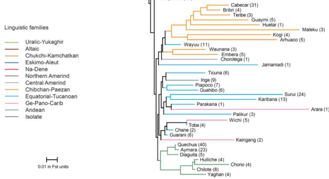
2.4.7 What about subspecies threshold? - AI gen
The claim that human racial groups meet the threshold for subspecies designation was addressed in the number density discussion above: global FST among continental human populations is roughly 0.07–0.15, well below the threshold of approximately 0.25 commonly cited for mammalian subspecies [Smith, Chiszar, & Montanucci 1997; Templeton 1998, 2013].
Templeton [2013] provides the most direct test of this claim. Using the same analysis method (AMOVA) applied to both species, he partitioned genetic variation in chimpanzees and humans into three components: variation among individuals within local populations, variation among local populations within the same race, and variation among races.
| Species | “Races” | Populations | Among individuals within populations | Among populations within races | Among races |
|---|---|---|---|---|---|
| Chimpanzees | 3 | 5 | 64.2% | 5.7% | 30.1% |
| Humans | 5 | 52 | 93.2% | 2.5% | 4.3% |
[Table: Templeton 2013, Table 2. AMOVA of genetic variation in chimpanzees and humans. Chimpanzee data from Gonder et al. 2011; human data from Rosenberg et al. 2002.]
Among chimpanzees, 30.1% of genetic variation falls between the three recognized subspecies — comfortably above the 25% threshold. Among humans, only 4.3% falls between the five traditional continental groupings — less than one-fifth of the threshold. Using the criteria applied to our closest living relative, chimpanzees have subspecies and humans do not [Templeton 2013].
The hereditarian may object that the 25% threshold is arbitrary. Templeton himself acknowledges this [Templeton 2013]. But the objection cuts the wrong way. The threshold was not invented for this comparison — it was calibrated against observed subdivision patterns across many vertebrate species and is the standard used under the U.S. Endangered Species Act for subspecies recognition in conservation biology [Smith, Chiszar, & Montanucci 1997; Pennock & Dimmick 1997]. It is the uniform criterion applied to every vertebrate species. The hereditarian who appeals to chimpanzee subspecies as evidence that small genetic differences can be biologically meaningful is appealing to a system that, when consistently applied, denies subspecies status to humans. And the margin is not close: humans are at 4.3%, not at 24%. Even if the threshold were arbitrarily halved to 12.5%, humans would still fail.
Moreover, the threshold criterion requires not only exceeding the quantitative bar but also sharp genetic boundaries separating the groups [Templeton 2013]. As we have seen, human genetic variation follows a smooth isolation-by-distance gradient with no sharp boundaries at all [Ramachandran et al. 2005]. Humans fail the subspecies definition on both counts — the quantity of differentiation and the pattern of differentiation — and neither failure is marginal.
Note that this is not the same as comparing FST values across species, which is methodologically illegitimate (as addressed in the next section). The subspecies threshold is a within-species criterion applied independently to each species. The question is not whether human FST is “smaller than” chimpanzee FST — it is whether human genetic variation meets the same standard for subspecies recognition that all other vertebrates are held to. It does not.
2.4.8 What about chimp-human FST being small too? (Verify)
Hereditarians sometimes object that chimpanzee-human genetic similarity is also high (approximately 98–99% at the aligned SNP level), yet the species are obviously very different—so perhaps the extreme genetic similarity among humans does not rule out large differences between populations either. A related version of this argument compares human-human FST to chimp-human FST and argues that both are “small.” This objection receives a full treatment in the section on quantifying population differences, where we show that it fails on multiple grounds: FST is a relative metric that cannot be meaningfully compared across species, the absolute genetic differences between humans and chimps are an order of magnitude larger than those between any two humans, and the kinds of variation differ—human-chimp differences concentrate in functional regions related to brain development and morphology, while human-human differences are overwhelmingly non-coding and functionally inconsequential. The human-chimp comparison is what selected divergence looks like; the human-human comparison looks nothing like it.
It is worth noting briefly why the cross-species FST comparison produces paradoxical results. Alcala and Rosenberg (2022, Philosophical Transactions of the Royal Society B) demonstrated that FST is mathematically constrained by allele frequency: with highly polymorphic markers like microsatellites, the mathematical ceiling on FST drops, which can produce the paradox where microsatellite FST between humans and chimpanzees appears lower than FST between chimpanzee subspecies. This is a mathematical artifact of how FST interacts with marker diversity, not a biological fact about species similarity [Alcala, N. & Rosenberg, N.A. (2022). “Mathematical constraints on FST: multiallelic markers in arbitrarily many populations.” Philosophical Transactions of the Royal Society B: Biological Sciences 377: 20200414.]. When appropriate corrections are applied, the paradox disappears. The hereditarian who cites raw cross-species FST to argue that small human FST can coexist with large differences is exploiting a mathematical artifact.
2.4.9 What about predicting ancestry from race? (Verify)
The previous objection asked whether genetic data can predict race. But the hereditarian can also argue in the reverse direction: if knowing someone’s race gives you useful information about their genetic ancestry, then race must be a meaningful biological category—it captures real biological information about the individual.
This argument has some empirical basis. At the continental level, racial labels do predict ancestry tolerably well. If someone in the United States self-identifies as non-Hispanic Black, you can predict with reasonable confidence that they carry majority sub-Saharan African ancestry. If they self-identify as non-Hispanic White, you can predict majority European ancestry. The ancestral clusters at the continental scale are large and well-separated, making coarse prediction from racial labels easier. Where race and ancestry have been historically stable—as they have been in the United States, where rigid social enforcement (anti-miscegenation laws, the one-drop rule, segregation) kept racial categories relatively aligned with broad continental ancestry for centuries—the prediction is better still.
However, this predictive correlation does not make race biologically real, any more than predicting someone’s native language from their country of birth makes language a biological category. The prediction works because the social categories were designed around coarse continental ancestry and maintained by social enforcement. What is doing the explanatory work is ancestry, not race. And the prediction degrades in exactly the ways a social category would degrade and a biological one would not.
First, the prediction breaks down at sub-continental scales. Knowing that someone is “Black” tells you very little about whether their ancestry is West African, East African, or Horn of Africa—populations that are, as we have seen, enormously genetically diverse, sometimes more different from each other than Europeans are from East Asians. Knowing someone is “White” tells you little about whether their ancestry is Northern European, Southern European, or Middle Eastern. The racial label is too coarse to capture the biologically relevant variation within it. This is not a minor limitation: continents are vast, and the genetic diversity they contain is enormous. A label that covers an entire continent’s worth of genetic variation and treats it as a single unit is discarding the overwhelming majority of the biological information it purports to capture.
Second, the prediction is unstable across societies. The same individual might be classified differently in different countries—“Black” in the United States, “pardo” (mixed) in Brazil, something else entirely in South Africa—and each classification would predict a different ancestry profile. A biological category should not change its predictive content when you cross a national border. Social races are often ill-defined or shifting even within a single society, making the prediction unreliable: as we saw in the prediction-from-genetics discussion, the “Rise of the Other” in U.S. Census data—from 48,604 individuals in 1950 to 27.9 million in 2020—means a growing fraction of the population does not fit the racial categories the prediction relies on. Ethiopian Americans, South Asian Americans, multiracial individuals, and many others occupy positions in ancestry space that the coarse racial labels cannot capture.
Third, and most tellingly, race is not the only social variable that predicts ancestry, and the others make the point obvious. In the United States, zip codes predict ancestry, because residential segregation means that knowing someone’s zip code tells you quite a lot about their likely continental ancestry proportions. Surnames predict ancestry. Religious affiliation predicts ancestry (as we saw with the Lebanese religious communities). Nobody argues that zip codes, surnames, or religious denominations are biological categories, even though all of them correlate with and predict ancestry. The fact that race also predicts ancestry places it in the same company: a social variable that correlates with biology because of how social structures are organized, not because the social variable is itself biological.
The bottom line: race is a noisy proxy for continental-scale ancestry, and a noisy proxy can have predictive value without being a natural kind. When researchers want to predict actual biological outcomes—disease risk, drug response, transplant compatibility—they increasingly use measured genetic ancestry rather than self-reported race, precisely because ancestry is the operative quantity and race is the lossy compression of it.
2.4.10 What about bone marrow transplants?
Sometimes in response to the claim that race is not a biological reality, the objection is raised that bone marrow transplants cannot reliably be made across racial lines — so race must, after all, be a biological category with medical consequences. In its strongest form, the argument runs: the medical establishment has every ideological incentive to treat race as fiction, yet bone marrow registries explicitly record race, match rates vary dramatically by ethnic background, and mixed-ancestry individuals face particular difficulty finding matches. If race weren't biologically real, the argument goes, none of this would be true.
This objection is an excellent test case for the distinction between race and ancestry, because it highlights something real and lets us see which framework — race as biology or race as a social construct correlated with ancestry — better predicts and explains the data. Bone marrow matching does correlate with self-identified race, and match probabilities do differ by ancestral background. A patient of European descent has roughly a 75–79% chance of finding an optimal matched donor in the U.S. registry; an African American patient's chances are closer to 29%; Hispanic and Asian/Pacific Islander patients fall in between at roughly 47–48% [Gragert et al. 2014; Be The Match / NMDP — verify current figures at publication time, as they shift upward as the registry grows]. These differences are not imaginary. The question is what explains them.
The answer is not that race is a biological kind but that bone marrow matching depends on Human Leukocyte Antigen (HLA)—a set of highly polymorphic immune-recognition genes on chromosome 6. Each person inherits one HLA haplotype from each parent; because HLA alleles are numerous and allele frequencies vary across populations, two unrelated individuals drawn from populations with similar ancestry are more likely to share haplotypes than two drawn from populations with different ancestry. Critically, the same HLA alleles are found across all human populations; what differs is their frequencies—continuous variation across populations, not discrete racial partitions. Notably, the registries themselves do not match donors and recipients by race. The actual match is determined entirely by HLA genetic testing. Self-reported race and ethnicity are collected as a search heuristic—a rough proxy used to predict likely HLA types and narrow the donor search—but the match decision is genetic [Hollenbach et al. 2015; NMDP]. A 2015 study examining how well self-identification predicts HLA found that no measure of self-identification corresponds completely with genetic ancestry, and recommended collecting donors' grandparents' geographic origins to improve prediction — moving the proxy closer to ancestry and further from race [Hollenbach et al. 2015]. Even the medical infrastructure built around bone marrow matching, in other words, treats race as a lossy shortcut for ancestry, not as the biologically operative category. As Dr. Jeffrey Chell, the head of the National Marrow Donor Program, put it: "Tell me where your ancestors lived 500 years ago, and I'll tell you who your potential donors are" [Washington Post, 2013 — verify exact date and full citation]. The operative concept is ancestry — where your ancestors lived — not race.
What does the race-as-biological-reality view predict? That racial categories carve nature at its joints such that same-race matches should generally succeed and cross-race matches should generally fail. What does the race-as-correlate-of-ancestry view predict? That the relevant variable is genetic similarity in HLA haplotypes, which tracks ancestry continuously. Since race correlates with ancestry, same-race matches will be more likely on average, but the operative quantity is haplotype identity, not racial category. Cross-race matches will happen whenever the right haplotype alignment exists, and the shortage of matches for non-white patients will primarily reflect the ancestry composition of the donor registry, not a biological barrier between races.
The data support the second prediction decisively, on five counts.
First, the sibling data. Full biological siblings — who share the same two parents, the same ancestry, and the same race on any definition — have only a 25% chance of being full HLA matches with each other. Fifty percent are half-matches, and twenty-five percent don't match at all. Roughly 70% of patients needing a transplant cannot find a match within their family and must search unrelated-donor registries [Gragert et al. 2014]. If race were the biologically relevant category for matching, same-race siblings would match reliably. They don't. Matching operates at a resolution far finer than race — a resolution at which the concept of race does no useful work.
Second, the registry composition data. The gap in match rates between white and non-white patients is driven substantially by who is in the donor registry. The Be The Match registry is approximately 67–74% white, while African Americans constitute only about 4–7% of registered donors — despite being roughly 13% of the U.S. population. Hispanic donors make up about 7–10% of the registry, and Asian donors about 7% [NMDP; Gift of Life — verify current composition at publication time]. This underrepresentation directly reduces the pool of potential HLA-matched donors available for minority patients: when fewer people of similar ancestry are in the registry, fewer haplotype matches can be found. As minority enrollment has grown over the past two decades, match rates for minority patients have risen accordingly — confirming that the barrier is a sampling problem in the donor bank, not a biological wall between races. The case of Jewish patients is instructive: in 1991, an Ashkenazi Jewish leukemia patient was told he had only a 5% chance of finding a match; a grassroots drive added over 60,000 Jewish donors to the registry, and today a Jewish patient's chance of finding a match is 75% [Gift of Life]. The barrier was never biology — it was registry representation. In addition, African-ancestry populations carry greater HLA diversity — more alleles, more rare haplotypes — than populations of European ancestry, which means that proportional representation alone may not close the gap entirely; a larger absolute number of African-ancestry donors per patient may be needed. This greater diversity is itself precisely what the nested subsets model of human genetic variation predicts: populations closer to the root of human dispersal retain more genetic diversity, including at the HLA loci.
Third, the cross-race matching data. Cross-race matches are not merely theoretically possible — they happen routinely in clinical practice. A 2014 University of Minnesota study examined 858 unrelated-donor transplant cases and directly compared outcomes when donor and recipient were of the same race versus different races. The study found no evidence that using a donor from a different race or ethnicity produced worse outcomes, and concluded that ethnic group matching should not be a factor in donor selection [Ustun et al. 2014 — verify full citation: PMC4064795]. This finding is incompatible with the race-as-biological-reality prediction that racial boundaries constitute biological barriers to transplantation. What matters is HLA match quality, regardless of the racial labels attached to donor and recipient.
Fourth, the identical-twin data point. The first successful bone marrow transplant, in 1956, was between identical twins, who share HLA essentially perfectly. Identical twins share race and HLA. Siblings share race but usually not HLA. Occasionally, unrelated people of different races share enough HLA for a match. Race is the variable that drops out of this chain; HLA identity is what matters.
Fifth, the cyclophosphamide data. A 2024 study found that with post-transplant cyclophosphamide, 7/8 mismatched transplants achieve outcomes comparable to full matches, expanding potential match rates for African American patients from roughly 29% to roughly 84%, and for Hispanic and Asian patients from under 50% to near 90% [Fingrut et al. 2024 — verify exact citation; figures drawn from secondary coverage in STAT News, July 17, 2024; locate primary paper in Journal of Clinical Oncology before publication]. If racial incompatibility were the biological barrier, no drug protocol could dissolve it. The barrier is a specific immune-rejection mechanism that medicine is learning to manage — not an impassable biological line between races.
What, then, about the argument that cross-ancestry marriage is imprudent — or, in the cruder version sometimes encountered online, that it produces children who are genetic misfits, unable to find a donor from either parent's group? The argument proves too much. Siblings of the same parents, the same ancestry, and the same race fail to match three times out of four. If matching difficulty were grounds to call a child a genetic misfit, three out of every four children would qualify. The practical response to registry gaps is not to restrict whose children are born but to diversify donor registries, which is precisely what the medical establishment has pursued, and with measurable success.
The distinction between race and ancestry allows us to predict and understand every feature of this phenomenon. Ancestry — continuous genetic similarity, measured in HLA haplotype frequencies — correctly predicts that matching will track ancestral proximity regardless of racial labels, that cross-race matches will occur when haplotype alignment exists, that the difficulty for minority patients is a registry sampling problem compounded by greater ancestral HLA diversity, and that matching resolution operates below the level of family, let alone race. Race as a biological category, by contrast, misled our understanding of what the matching barrier actually is, and made the incorrect prediction that cross-race donors cannot exist.
2.5 Genetic Variation 102: Quantifying Population Differences
We have seen that race is not a biological entity—it is a social construct. However, social constructs can have average genetic differences. Any two populations can have average genetic differences. Because of how poor a proxy race is for biology, we would expect there to be little genetic differences on average. However, average population differences is a distinct question from whether race is a biological entity. To understand how to answer that question, we must turn again to genetics to understand how genetics gives rise to observable traits and then how to quantify differences in traits.
2.5.1 Genotype and Phenotype
The variation that we have thus far been discussing is genetic variation—this is variation in the human genome. The alleles that an individual carries at one or more locations in the genome are known as the genotype. (Recall that at each variable position, an individual carries a combination of alleles—AA, AG, or GG, for example. That combination is the individual’s genotype at that position; across many positions, the collection of such combinations is the individual’s genotype across those positions.) The genotype is distinct from the genome: the genome is the entirety of an individual’s DNA while the genotype is the individual’s genetic makeup at the particular positions being examined.35 An individual’s genetics expresses itself as an observable trait. We call the observable traits the phenotype. The phenotype is not solely an individual’s genetics expressing themselves but the genetics in combination with environment together produce the phenotype. The environment is simply effects on traits that do not come from an individual’s genome.
Quantitative traits are those that can be described by assigning a (continuous) numerical value. It turns out that a simple additive model goes far in explaining human traits. The idea is that each gene either contributes or takes away from a trait’s value. Adding all of these and adding the environment (which also could add or take away from a trait’s value) then produces the final phenotype value. Because phenotypes are produced in part from the environment, it is possible for the same genotype to produce a different phenotype or distinct genotypes to produce the same phenotype. For an example, an individual might be genetically predisposed to be tall. However, the individual does not have good nutrition (environment) and ends up at an average height. Meanwhile, another individual is genetically predisposed to be short but has excellent nutrition and likewise ends up at an average height. Genes and environments are independent and different combinations can end up at the same trait value (e.g., lower genetics plus good environment; higher genetics plus poor environment).
(AI gen; verify) Genes can also interact with other genes (called epistasis, or GxG) or with the environment (GxE), and individual alleles can exhibit dominance (think dominant versus recessive from Punnett squares). However, a foundational result in quantitative genetics is that for complex traits governed by many genes, additive genetic variance—the variance attributable to the independent, additive effects of individual alleles—accounts for the large majority of total genetic variance, typically over half and often much more, even when substantial epistasis and dominance exist at the level of individual gene pairs [Hill, Goddard, & Visscher, “Data and Theory Point to Mainly Additive Genetic Variance for Complex Traits,” PLoS Genetics 4(2): e1000008, 2008]. The reason is intuitive: when thousands of genes each contribute a small effect to a trait, any specific interaction between two of them is swamped by the independent contributions of the other thousands. The interaction affects the phenotype of the rare individual who carries that specific combination, but when averaged across the population, its contribution to the total variance is tiny. Moreover, when allele frequencies are far from 50%—as most are, with many variants being rare—the additive component of even a strongly epistatic locus dominates the population-level variance, because most individuals carry only one of the interacting alleles, not both [Hill et al. 2008]. Gusev has illustrated this empirically, showing that rare variant effects and polygenic scores combine approximately linearly across multiple traits, with no detectable interaction [Gusev, “Beneath the surface of the sum,” The Infinitesimal (Substack), August 27, 2025]. The practical consequence is that the simple additive model—in which each allele contributes independently to the trait, and the total genetic effect is the sum of individual contributions—is an excellent approximation for complex traits at the population level, even if the underlying biology involves extensive gene-gene interaction at the molecular level. This distinction between individual-level epistasis and population-level additivity is important to keep in mind throughout the rest of this paper.
Moreover, as noted before, some regions of the genome are coding and others are non-coding. The vast majority of human genetic variation falls in non-coding regions and is spread throughout the genome. Most of this variation has no known effect on any trait. However, some non-coding variation acts as regulatory elements, controlling how strongly genes are expressed—turning them up or down, or on or off in particular tissues—rather than coding for a protein that directly influences a trait. The genome-wide association studies used to identify trait-affecting variants sample positions distributed across the entire genome—coding, regulatory, and other non-coding regions alike—so the search for trait-affecting variants is not restricted to the small coding fraction.
Because genes and environments can vary for individuals, the phenotypes in a population likewise can vary, resulting in phenotypic variation. The phenotypic variation is a result of the genetic and environmental variation in the population.
2.5.2 How Phenotypic Variation is Distributed
We saw in the Genetic Variation 101 section that genetic variation is distributed continuously across geography and that most of it is found within populations rather than between them: 85% within, 15% between. Perhaps surprisingly, observable traits—the phenotypes produced by genetic variation—follow many of the same patterns.
First, phenotypic traits are clinally distributed: they vary in smooth geographic gradients rather than jumping from one value to another at population boundaries. If you were to travel from Scandinavia south through Europe to North Africa, you would not see skin color suddenly change at some border. You would see it gradually, continuously darken as you moved south. Cross the Mediterranean and continue through the Sahara and into West Africa, and the gradient continues. There is no line where “light” ends and “dark” begins—only a smooth continuum. Jablonski and Chaplin used NASA satellite data on surface UV radiation levels to predict indigenous skin colors at every point on the globe, and their predictions matched observed skin tone distributions with remarkable precision [Jablonski & Chaplin, “The evolution of human skin coloration,” Journal of Human Evolution 39 (2000): 57–106; Chaplin, “Geographic distribution of environmental factors influencing human skin coloration,” American Journal of Physical Anthropology 125 (2004): 292–302]. The resulting map shows a smooth, continuous gradient from equator to poles.
[Graph: Global skin color map — the Jablonski & Chaplin predicted skin color map or the Biasutti map of indigenous skin colors. These are heatmap-style geographic representations showing the smooth gradient. Available from the Museum of Us (Google Arts & Culture), the Smithsonian Human Origins page, or standard biological anthropology textbooks.]
Skull measurements are likewise clinally distributed. Within Europe alone, cranial morphology varies along a northwest-to-southeast gradient that closely tracks genetic population structure [Betti et al., “A geographic cline of skull and brain morphology among individuals of European ancestry,” Human Biology 82 (2010): 595–606 [verify journal details]]. Globally, craniometric distances between populations track geographic distances much as genetic distances do [Relethford, “Global patterns of isolation by distance based on genetic and morphological data,” Human Biology 76 (2004): 499–513]. There is no point on the map where skull shape suddenly shifts from one “type” to another. Skull shape and size—the very measurements that 19th-century race scientists used to construct racial hierarchies—form gradients, not discrete types.
Blood group frequencies make the clinal point in a different way. The ABO blood group system is not a continuously varying trait within an individual—you are type A, B, AB, or O. However, the frequencies of these blood types across populations vary continuously in geographic gradients. Blood group B, for instance, reaches its highest frequency in Central Asia, is moderately common in the Middle East and East Asia, drops off across Europe from east to west, and was essentially absent in pre-contact Indigenous American and Australian populations [Mourant, Kopeć & Domaniewska-Sobczak, The Distribution of the Human Blood Groups and Other Polymorphisms, 2nd ed. (1976); Cavalli-Sforza, Menozzi & Piazza, The History and Geography of Human Genes (1994)]. Blood group A is most common in parts of Europe and, perhaps unexpectedly, among some Australian Aboriginal populations. These frequency gradients do not respect racial boundaries: populations assigned to the same “race” can have very different blood group profiles, and populations assigned to different “races” can have similar ones.
[Graph: Global maps of ABO allele frequencies — heatmap-style geographic maps showing the distribution of A, B, and O alleles globally. Three small maps (one per allele) showing how each allele’s gradient runs in a different geographic direction. Available from Cavalli-Sforza et al. (1994) or biological anthropology textbooks.]
That last observation—that blood groups carve up humanity differently than skin color does—is not a quirk of blood groups. It is the general pattern. Different traits have different geographic distributions. The anthropologist Frank Livingstone famously wrote, “There are no races, only clines” [Livingstone, “On the non-existence of human races,” Current Anthropology 3, no. 3 (1962): 279]. Part of what he meant was that skin color varies along a north-south gradient, blood group B along an east-west gradient, nose shape with temperature and humidity, and so on. Each trait has its own clinal distribution, and these distributions do not line up. Biologists call this non-concordance: traits are observed to vary independently in their geographic distributions rather than clustering together [Brace, “A nonracial approach towards the understanding of human diversity,” in Montagu, ed., The Concept of Race (1964): 103–152]. If you classified people by blood type instead of skin color, you would draw different boundaries. If you classified by nose shape, different ones again. No single trait—and no set of visible traits—sorts humanity into the same groups as any other.
Second, when the distribution of phenotypic variation is quantified—how much lies within populations versus between them—most traits follow the same pattern as genetic variation. Relethford applied quantitative genetic methods to a large global craniometric dataset (57 skull measurements from populations across the world, originally collected by W. W. Howells) and found that roughly 13% of the total craniometric variation lies between major geographic regions, with the remaining 87% within regions [Relethford, “Craniometric variation among modern human populations,” American Journal of Physical Anthropology 95 (1994): 53–62; Relethford, “Apportionment of global human genetic diversity based on craniometrics and skin color,” American Journal of Physical Anthropology 118 (2002): 393–398]. These numbers match the 10–15% between-group variation found with genetic markers almost exactly. If you lined up skull measurements from people across the world, the distributions would overlap massively—the variation between any two individuals in the same population dwarfs the average difference between populations.
[Graph: Craniometric overlap — overlapping distributions of a craniometric measurement (e.g., cranial capacity or cranial breadth) across populations, showing the large within-group spread and the modest between-group shift. Howells’ dataset is publicly available and could generate these histograms.]
Skin color, however, is strikingly different. In the same study, Relethford found that for skin color, the apportionment is essentially reversed: roughly 88% of global skin color variation lies between major geographic regions, with only about 9% within local populations [Relethford 2002]. Skin color is, among well-studied traits, a dramatic outlier in its between-group variation. We will return to why after discussing how selection operates on traits, and we will see that the explanation has important implications for what skin color can and cannot tell us about deeper biological differences.
2.5.3 Polygenicity
[Source on selection being rare and rare alleles being more recent and localized than common alleles: https://nap.nationalacademies.org/read/26902/chapter/4#29]
Some quantitative traits are determined by single genes. Perhaps you have heard of “The gene for this or that.” We call these traits monogenic. It turns out that these traits often tend to be disease traits: a single gene is often a rare and harmful mutation.
Other quantitative traits are controlled by multiple genes and locations in the genome. These traits are polygenic. It turns out that most human traits are polygenic, and human behavioral traits (traits dealing with human behavior, like educational attainment (i.e., years of formal education), IQ, psychological conditions like depression or schizophrenia, occupation, income) are even more polygenic, controlled by even more sites in the genome (a trait’s polygenicity refers to the number of sites in the genome that contribute to the trait)! These multiple genes act together to produce more or less of a trait, as we described when discussing the additive model. Polygenic traits in humans are often controlled by hundreds or thousands of locations spread throughout the genome, each having just a tiny effect on the trait’s expression and then adding up to the final resulting gene expression (called the polygenic score), which in combination with the environment produces the final trait value. We call such traits that are determined by multiple genetic and environmental factors complex traits, and most traits in humans are complex traits.
Because the polygenic score is a sum over hundreds or thousands of tiny contributions, there are vastly more allelic combinations that produce any given score than there are possible scores—two individuals can carry completely different sets of trait-influencing variants and still arrive at the same genetic value. This is a basic combinatorial property of additive models: if a trait is influenced by a thousand loci, there are astronomically many ways to reach a score of, say, 500 out of 1,000. We will see downstream consequences of this many-to-one property when we examine how selection operates on polygenic traits and how trait differences between populations relate to genetic differences.
Recall that SNPs drive most traits. A SNP is a single-letter variation at one position in the genome; a gene—which typically spans thousands of letters—may contain many SNPs. So when genome-wide association studies identify hundreds of SNPs associated with a trait, those SNPs are distributed across a smaller number of genes. As an example of how polygenic traits can be, consider skin color. Skin color is controlled by the amount of melanin produced and is influenced by at least 15–20 confirmed genes, with over 500 associated SNPs identified across multiple genome-wide association studies [Pospiechet al. 2014, Forensic Science International: Genetics; Walsh et al. 2017, Human Genetics; Lona-Durazo et al. 2019, BMC Genomic Data]. Each of these SNPs nudges melanin production slightly up or slightly down; their effects add together to produce the final skin tone. Moreover, studies in African populations have shown that even these confirmed loci explain only a small fraction of the heritable variation in skin color, meaning many additional contributing loci remain to be discovered [Crawford et al. 2017, Cell; Martin et al. 2017, Cell]. Mouse models of pigmentation identify over 370 relevant loci, many with human homologues, suggesting the full genetic architecture of human skin color is substantially more complex than currently characterized [IFPCS and ESPCR mouse pigmentation database; see also Baxter & Pavan 2013, Pigment Cell & Melanoma Research [verify]].
Because many traits are highly polygenic, there is no “gene for” many traits. Perhaps you have heard how we will find a “gene for” this or that: this is known as a “candidate gene” and was an approach in population genetics for some time. It was thought at most there were only a handful of genes that contributed to a trait. However, the discovery that traits were so highly polygenic showed this to be incorrect: rather there is more or less of a trait (its genetic component anyway) depending on how much or how little genes are expressed.
[[Remove below after making sure all information in it is already in this section]]
[Altogether, genetic variation tends to result in genes expressing themselves more or less. In particular, SNPs—which drive most traits—tend to have small individual effects on gene expression. A variation in a single site will result in the gene expressing itself a little more or a little less, but in aggregate, there are thousands of SNPs which have tiny effects that add together to result in the final level of gene expression. All of this genetic variation in combination with environmental factors eventually results in variation in phenotype. And it turns out that many traits are polygenic—controlled by multiple genes; sometimes hundreds of genes, acting together to produce more or less of a trait, e.g., skin color is controlled by the amount of melanin produced and is controlled by ~400 genes and thousands of SNPs (https://www.gbhealthwatch.com/Trait-Skin-Color.php#:~:text=Human%20skin%20color%20is%20a,color%20in%20human%20and%20mice.). There is no “gene for” many traits but rather more or less of a trait depending on a number of genes and how much they are expressed.]
2.5.4 Selection
Natural selection operates on traits to drive them to fitness values, and by driving the traits to those values, the genetic variation behind the trait gets dragged along for the ride, resulting in changes in allele frequencies in a population. It turns out that there are different ways selection can do that.
Directional selection pushes a trait in one direction. Positive directional selection pushes a trait to higher values because those higher values are beneficial for fitness; negative directional selection (also called purifying selection) pushes against alleles with harmful effects, keeping them rare. Positive directional selection is what most people think of when they hear "natural selection": a trait becomes more common because it helps survival or reproduction.
Stabilizing selection is different and arguably more important for our purposes. In stabilizing selection, there is an optimal trait value for fitness, and deviation in either direction results in reduced fitness. An example is birth weight in humans: neonates below 3 kg face elevated mortality from underdevelopment; neonates above 4.5 kg face elevated mortality from birth complications. The intermediate range has the best survival outcomes. Stabilizing selection does not push a trait in any particular direction—it holds it in place around an optimum. This distinction turns out to be critical: most complex human traits appear to be under stabilizing selection, not directional selection (Simons, Bullaughey, Hudson & Sella 2018, PLoS Biology; Sanjak et al. 2018, PNAS; Hayward & Sella 2022, eLife). We will return to why this matters when we discuss population differences.
Selection acts in response to selection pressure: the pressure could be a natural change in the environment or other factors, e.g., maybe a social-cultural phase sweeps through a population that makes everyone want to marry those with blue eyes. The selection pressure could be applied transiently—just for a time—after which the trait may settle back down to its original value or now oscillate about a new trait average. After the selection pressure settles down, drift may take over. Selection pressure could also be constantly applied, such as selection against traits with harmful effects, e.g., disease from genetic mutation. Multiple different selection pressures could be applied transiently or constantly. It is also possible that a trait is optimal in multiple environments and conditions and as a result multiple populations will converge upon the same trait value (called "convergent selection").
Divergent selection is worth singling out because it is what the hereditarian argument ultimately requires. Divergent selection is directional selection favoring different trait optima in different populations—selection that pulls populations apart. If one population faces environmental pressure favoring higher cognitive ability and another faces pressure favoring lower cognitive ability (or faces no such pressure at all), that would be divergent selection. Divergent selection is one specific kind of adaptation; it should not be confused with adaptation in general, which can be convergent (multiple populations adapting toward the same optimum) or stabilizing (holding at an existing optimum). The hereditarian argument requires divergent selection on cognitive traits between continental populations. As we will see, this specific claim has not been demonstrated.
As concrete examples of what directional selection between populations actually looks like, consider two well-studied cases: lactase persistence and the sickle cell allele. Lactase persistence—the ability to digest milk sugar (lactose) into adulthood—is at high frequency in Northern European dairying populations, East African pastoralist groups (such as the Fulani, Maasai, and Tutsi), and certain Middle Eastern and South Asian pastoralist communities (such as the Bedouin, Toda, and Gujjar). These populations span multiple continents and what would conventionally be called multiple races, but they share a history of herding livestock and consuming milk. The trait tracks subsistence strategy—pastoralism—not continental ancestry. Populations within the same racial category but without pastoralist traditions (most East Asians, many West African agricultural groups) have low lactase persistence [Tishkoff et al., “Convergent adaptation of human lactase persistence in Africa and Europe,” Nature Genetics 39 (2007): 31–40; Gerbault et al., “Evolution of lactase persistence: an example of human niche construction,” Philosophical Transactions of the Royal Society B 366 (2011): 863–877]. Moreover, the trait arose independently from different mutations in European and African populations: the European variant (–13910T upstream of the LCT gene) is distinct from the East African variants (–14010C, –13915G, –13907G). Natural selection converged on the same phenotype through separate genetic paths in populations under similar ecological pressure [Tishkoff et al. 2007; Ranciaro et al., “Genetic origins of lactase persistence and the spread of pastoralism in Africa,” American Journal of Human Genetics 94 (2014): 496–510]. Race predicts neither who has the trait nor what genetic variant underlies it.
[Graph: Lactase persistence global distribution map — use the map from Gerbault et al. (2011) or the map reproduced in Tishkoff et al. (2007) or the Itan et al. map, showing frequency of lactase persistence phenotype globally. The key visual is that the trait appears at high frequency in Northern Europe AND East Africa AND parts of the Middle East—populations that would be assigned to different races but share pastoral histories.]
The sickle cell allele (HbS) tells a similar story. It is common in sub-Saharan Africa, but also in parts of the Mediterranean (Greece, southern Italy, Turkey), the Middle East, and India—populations that cross conventional racial categories. Its distribution maps onto historical malaria endemicity: wherever Plasmodium falciparum malaria was historically a major cause of mortality, the sickle cell allele rose in frequency because carriers (heterozygotes) have partial resistance to malarial infection. Piel et al. produced the first detailed global map of HbS allele frequencies using a Bayesian geostatistical framework and confirmed the geographical correspondence with pre-intervention malaria transmission zones at a global scale [Piel et al., “Global distribution of the sickle cell gene and geographical confirmation of the malaria hypothesis,” Nature Communications 1, article 104 (2010)]. A trait commonly thought of as “an African disease” is in fact a malaria adaptation found wherever malaria was historically endemic, regardless of continental ancestry.
Graph: Sickle cell global distribution overlaid or side-by-side with historical malaria endemicity — use the maps from Piel et al. (2010), which show HbS allele frequency alongside pre-intervention malaria zones. The visual parallel is immediately striking.]
These examples are worth keeping in mind as we turn to the hereditarian argument about cognitive traits. The hereditarian claim requires divergent selection—selection pulling populations apart on cognitive ability. Lactase persistence and sickle cell show us what directional selection that produces between-population differences actually looks like when it occurs: it follows identifiable ecological pressures, it crosses racial boundaries, it produces detectable molecular signatures, and its genetic basis can be pinpointed. Among populations under the same pressure the pattern is convergent; relative to populations without that pressure, the result is divergence from them. Either way, the trait tracks ecology, not race. As we will see, the claimed cognitive differences between racial groups display none of these features.
At the level of individual genetic variants, selection can act in different ways as well. A hard sweep occurs when selection drives a new beneficial allele from very low frequency all the way to fixation in a population, sweeping away nearby genetic variation in the process. Hard sweeps leave distinctive signatures in the genome—reduced genetic diversity around the selected site—and are relatively easy to detect. A soft sweep occurs when selection acts on an allele already present in the population at appreciable frequency, increasing it but not necessarily to fixation. Soft sweeps are harder to detect because their genomic signature is subtler. Selection may act on individual loci in the genome (single-locus selection), or it may operate on many loci simultaneously (polygenic selection).
Polygenic selection - AI gen is especially relevant for behavioral traits. Because traits like educational attainment and cognitive ability are influenced by thousands of genetic variants each with tiny effects, selection on these traits would not produce dramatic hard sweeps at individual loci. Instead, it would produce subtle, coordinated shifts in allele frequencies across many loci—each shift too small to detect individually, but potentially adding up to a meaningful change in the trait's average value. This is what happens in animal breeding: breeders do not wait for new mutations; they select on standing variation across many loci simultaneously. The question for the hereditarian argument is whether this kind of selection has occurred differentially between human populations on cognitive traits. Detecting such selection in humans is methodologically difficult, and we will examine the evidence directly.
There is an important corollary of polygenic architecture that is worth pausing on: polygenic traits are remarkably resistant to selective culling—the removal of individuals at one extreme of the distribution. For a monogenic trait—a disease caused by a single gene—selection can be brutally efficient. If every carrier is removed from the breeding population, the causal allele disappears in a single generation. But for a trait influenced by thousands of variants, each contributing a tiny effect, the picture is entirely different.
The reason is that selection operates on the phenotype—the total trait value—not on individual alleles. When the trait is polygenic, each individual allele contributes so little to the phenotype that selection can barely distinguish carriers from non-carriers. Consider a simplified example: suppose aggression is influenced by 1,000 genes, each with a tiny effect, and you remove the most aggressive 5% of the population each generation. The individuals you remove happen to carry a slightly higher-than-average number of “aggression-increasing” alleles—say 520 out of 1,000 instead of the population average of 500. But the people just below the threshold you set—the ones who survive—might carry 515 or 510 of the same alleles. They share nearly all the same aggression-increasing variants; they simply drew a slightly less extreme combination. When those survivors reproduce, their alleles reshuffle into new combinations, and some of the offspring will again carry 520 or more—landing right back above the threshold. The extreme combinations are culled each generation, but the alleles that compose them remain in the population at nearly the same frequencies, because, at this intensity of selection, each individual allele contributes too little to the phenotype for its frequency to shift meaningfully.
There is a second reason culling fails in practice, beyond the allele-persistence problem. In a controlled breeding experiment, the environment is held constant, so phenotypic differences reflect genetic differences with reasonable fidelity. In a real human population, people are not raised in identical environments. When a eugenics program selects against a phenotype like criminality, it is selecting on a trait shaped by both genes and environment. Some of the individuals removed from the breeding population are at the aggressive extreme for largely environmental reasons—childhood trauma, lead exposure, neighborhood violence—while carrying genotypes near the population average. Others who pass the cutoff carry high genetic liability that was never expressed because their environment was favorable. The phenotypic cutoff is therefore a blurred proxy for the underlying genetic variation. This blurring reduces the effective selection differential below the nominal cutoff, further weakening an already-weak selection regime.
Gusev has demonstrated this formally through multi-generational simulations. For a monogenic trait with approximately 1% incidence, removing all affected individuals each generation drives the incidence to near-zero within two generations. For a polygenic trait with the same starting incidence and heritability, the same selection barely moves the incidence—reducing it from about 1% to only about 0.75% over five generations—because the causal alleles remain in the population [Gusev, “What happens to heritable conditions across generations?,” The Infinitesimal (Substack), December 26, 2024]. [Figure: Gusev’s monogenic vs. polygenic selection simulation graph, showing incidence over 5 generations. Available from the cited Substack post.] Gusev’s formal simulations model threshold traits specifically (traits that are either present or absent, depending on whether an underlying continuous liability exceeds a threshold). But as we have seen—and as Gusev has stated in summarizing the general principles—the core insight applies to all polygenic traits, continuous and threshold alike: “(1) selection on a heritable trait in a controlled environment will produce a response, but the long-term response is very hard to predict (other than it is almost certainly very slow); (2) you cannot breed out a polygenic trait because the causal alleles exist in all humans” [Gusev, X/Twitter thread, March 16–17, 2026 [note to self: reference the specific X thread URL]].
For continuous traits like height and cognitive ability, the implication is the same: selection can shift the population mean, but it cannot eliminate the underlying alleles. Each generation, recombination reassembles them into new combinations, reproducing the full range of phenotypic values. Mutation continuously replenishes variation. And pleiotropy—the fact that many alleles affect multiple traits simultaneously—tends to create opposing selection pressures that prevent any one allele from being driven to zero. Intense artificial selection in a controlled environment—such as what animal breeders practice—can shift the mean substantially by changing allele frequencies, because the breeder controls who reproduces and the uniform environment ensures that phenotypic selection tracks genetic variation accurately.36 But for selection at the extremes of a natural human population—the eugenics scenario—the selection intensity is far too weak and the phenotypic signal far too noisy to produce meaningful change. The causal alleles cannot be bred out because they exist in all of us. This is worth keeping in mind as we turn to questions about population differences in complex traits.
2.5.5 Skin Color, Selection, and Non-Concordance
We noted earlier that skin color’s apportionment of variation is strikingly different from that of genetic markers or skull measurements: roughly 88% of skin color variation lies between major geographic regions, compared to only 10–15% for genetic markers and ~13% for craniometric traits [Relethford 2002]. Now that we have discussed selection, we can see why.
Skin color is under strong directional selection driven by ultraviolet radiation. Populations near the equator experience intense UV, which selects for darker pigmentation to protect against folate degradation and DNA damage. Populations at higher latitudes experience less UV, which selects for lighter pigmentation to allow sufficient vitamin D synthesis [Jablonski & Chaplin, Journal of Human Evolution 39 (2000): 57–106; Jablonski, “The evolution of human skin and skin color,” Annual Review of Anthropology 33 (2004): 585–623]. This is directional selection that is geographically structured—the selection pressure itself varies clinally with latitude—and it has pushed skin color to diverge between populations far beyond what genetic drift or neutral processes would produce. Because UV intensity tracks latitude rather than continental ancestry, skin color cuts across racial boundaries: equatorial populations in sub-Saharan Africa, South Asia, and Melanesia converge on similarly dark skin tones despite being among the most genetically distant populations on earth, while high-latitude populations in Europe and East Asia have independently evolved lighter skin through partially distinct genetic pathways [Norton et al., “Genetic Evidence for the Convergent Evolution of Light Skin in Europeans and East Asians,” Molecular Biology and Evolution 24, no. 3 (2007): 710–722 [verify full citation]]. Skin color groups people by latitude, not by race.
For traits not under strong directional selection, theory predicts that polygenicity should not amplify between-group differences. Edge and Rosenberg showed mathematically that for a selectively neutral, additive, polygenic trait, the expected phenotypic difference between populations is comparable in magnitude to the genetic difference at a single locus—regardless of how many loci influence the trait [Edge & Rosenberg, “Implications of the apportionment of human genetic diversity for the apportionment of human phenotypic diversity,” Studies in History and Philosophy of Biological and Biomedical Sciences 52 (2015): 32–45; Edge & Rosenberg, “A General Model of the Relationship between the Apportionment of Human Genetic Diversity and the Apportionment of Human Phenotypic Diversity,” Human Biology 87, no. 4 (2015): 313–337]. The reason is that for a neutral trait, the direction of allele frequency differences at each locus is random: at some loci the allele that increases the trait is more common in one population, at others it is more common in the other. These random differences cancel out across loci rather than accumulating. This prediction matches the craniometric data: skull measurements, which appear to be largely under stabilizing rather than directional selection, show the same 85/15 apportionment as genetic markers.
What does this mean for the significance of skin color?
Skin color is the single most visible human phenotype and the trait most strongly associated with racial categories in the popular imagination. It is also the most extreme outlier in its between-group variation among well-studied phenotypes. Most phenotypic traits—skull measurements, body proportions, physiological characteristics—show the pattern of most variation lying within groups. Skin color shows the reverse. The trait we use most readily to sort people into races is the trait least representative of overall human phenotypic variation. Our eyes are drawn to the exception.
Moreover, skin color is independent of virtually all other phenotypic and genetic traits (the obvious exceptions being other pigmentation traits such as eye and hair color, which share some of the same underlying genes and therefore tend to correlate at the population level, though even these can dissociate in individuals, as we will see). The technical term is non-concordance: we noted earlier that different traits have different clinal distributions, but now we can see why—each trait’s distribution is shaped by its own history of selection pressures (or drift), and these pressures are largely unrelated to each other. The selection pressure on skin color (UV radiation) has nothing to do with the selection pressures on, say, blood group frequencies (which may involve pathogen resistance) or lactase persistence (which involves pastoralism). Because the genetic variants controlling skin color are a small and largely independent set of loci, a person’s shade tells you about those handful of pigmentation genes and remarkably little about the other 99.99% of their genetic variation.
This independence is not merely theoretical. In Cape Verde, an island population with both West African and European ancestry, Beleza et al. found that skin color correlated poorly with genome-wide ancestry at the individual level—and that individuals with dark skin and blue eyes were not uncommon [Beleza et al., “Genetic architecture of skin and eye color in an African-European admixed population,” PLOS Genetics 9, no. 3 (2013): e1003372]. Studies of Brazilians have likewise found that molecular ancestry is a poor predictor of skin color at the individual level [Parra et al., “Color and genomic ancestry in Brazilians,” PNAS 100 (2003): 177–182 [verify citation]]. The genes that make someone dark-skinned or light-skinned are involved in melanin synthesis and transport—a biological pathway with no established connection to the genetic architecture of other trait systems like cognition, body size, or disease susceptibility.
The visible differences between human populations are real, but they are a poor guide to deeper biological differences. The deeper pattern—which we see in genetic markers, in skull measurements, and in the theoretical predictions for traits not under strong selection—is one of overwhelming overlap. We will see this principle tested directly when we examine the specific claims hereditarians make about intelligence, where the question is precisely whether cognitive traits have been under the kind of strong divergent selection that could produce a skin-color-like exception to the general pattern. As we saw with lactase persistence and sickle cell, when such selection does occur, it follows ecology rather than racial categories, and it leaves detectable molecular signatures.
2.5.6 A Note on Skin Color Inheritance
We have seen that skin color is polygenic and additive: many genes each contribute a small amount to melanin production, and their effects add up. This has an important consequence for how skin color is inherited—a consequence that is often misunderstood.
Skin color inheritance is not like mixing paint. If you mix white and brown paint, you get a uniform tan, and mixing two cans of that tan produces the same tan forever after. But genes do not blend; they segregate—as we saw in the section on recombination, each parent passes on a random half of their alleles at each locus, and the child’s genome is a fresh shuffle of the parental deck. For a polygenic trait like skin color, this means the children of two intermediate-toned parents do not all come out the same shade. Instead, their skin tones follow a distribution—a range of possible values centered near the parental average, with some children noticeably lighter and some noticeably darker. Each child receives a different random draw of pigmentation alleles from each parent, and with at least 15–20 contributing genes, the number of possible allele combinations is enormous.
To see how this works concretely, consider a simplified model with just three genes, each with two alleles—a “dark” allele that adds a unit of melanin and a “light” allele that does not. (The real system involves at least 15–20 genes, but the three-gene model illustrates the principle.) A parent who is maximally dark carries all six dark alleles: AABBCC. A parent who is maximally light carries all six light alleles: aabbcc. Their children—the first generation—all receive three dark and three light alleles (AaBbCc) and are intermediate in skin tone. So far, this looks like blending. But now consider what happens when two of these intermediate individuals have children. Each parent passes on a random allele at each of the three genes. The possible combinations in the second generation range from zero dark alleles (aabbcc—lightest possible) through three dark alleles (the intermediate parental tone) to six dark alleles (AABBCC—darkest possible). The distribution follows the binomial pattern: out of 64 equally likely genotype combinations, 1 will be lightest, 6 slightly darker, 15 darker still, 20 at the intermediate parental tone, 15 lighter than intermediate, 6 lighter still, and 1 lightest. Most children cluster near the parents’ intermediate shade, but the full range from lightest to darkest is possible. With the real system of 15–20 or more genes, the distribution is smoother and the extremes are rarer, but the principle is the same: each child is an independent draw, siblings can differ substantially from one another, and neither parent’s phenotype “dominates.”
[Figure: The three-gene model of polygenic skin color inheritance, showing the F2 distribution from two intermediate (AaBbCc) parents. Seven phenotypic classes (0 through 6 dark alleles) with frequencies 1:6:15:20:15:6:1, displayed as a histogram with skin tone shading for each bar. For an open-access classroom version of this model, see HHMI BioInteractive, “Understanding Variation in Human Skin Color” (2017, revised), available at biointeractive.org under CC BY-NC-SA 4.0. Standard genetics textbooks (e.g., Griffiths et al., Introduction to Genetic Analysis; Pierce, Genetics: A Conceptual Approach) include similar figures. A figure drawn for this paper would avoid copyright issues entirely.]
In practice, substantial variation among siblings is common, not rare. In families where the parents are of different ancestry—or where both parents carry a mix of light and dark alleles from prior admixture—the children can range from very light to quite dark. Each child is an independent draw from the distribution, so with several children, seeing a wide spread of skin tones across the siblings is expected. This is especially visible in families where one parent is white and the other is mestizo (mixed European and Indigenous American ancestry): the mestizo parent already carries many light-skin alleles from their European ancestry, and with a white parent contributing all light alleles, a substantial fraction of the children may be as light-skinned as any European. The probability depends on how many dark alleles the mestizo parent carries—but in many cases, a quarter or more of children will inherit few or no dark alleles from that parent and be phenotypically indistinguishable from the white parent, while their siblings may be noticeably darker. The genes are segregating exactly as the additive model predicts.
Moreover, epistatic interactions between pigmentation genes—where the effect of one gene depends on what alleles are present at another—can widen this distribution beyond what the simple additive model alone predicts, occasionally producing phenotypes more extreme than either parent [Pospiech et al. 2014, Forensic Science International: Genetics; Branicki et al. 2009, Annals of Human Genetics [verify]]. Such epistatic effects are possible for skin color because it is governed by a relatively small number of genes with individually large effects—a context where specific allele combinations can matter. For highly polygenic traits like cognitive ability, governed by thousands of genes each with tiny effects, individual-level epistasis exists but averages out at the population level, as discussed earlier in the genetics sections. The Sandra Laing case in South Africa is a well-known example of extreme recombination: a phenotypically dark-skinned child born to two phenotypically white Afrikaner parents, confirmed by genetic testing to be her biological parents. Laing’s parents carried African-ancestry alleles at pigmentation loci that, by chance, co-segregated in her—producing a phenotype neither parent expressed [see Judith Stone, When She Was White: The True Story of a Family Divided by Race (2007) [verify]].
The folk-genetic belief that “dark-skinned genetics dominate” in mixed offspring is a misperception. Mixed children are, on average, intermediate in skin tone between their parents, and their siblings vary around that intermediate in both directions—exactly as the additive model predicts. The perception of dominance likely arises from a combination of factors: perceptual asymmetry (mixed offspring are darker than the white parent, which makes it appear from the white parent’s perspective that “the dark won”), confirmation bias (darker children may be noticed or remembered more readily in contexts where dark skin is socially marked), and in the American context, the one-drop rule, which classified mixed children as black regardless of actual skin tone—a convention codified in statutes like Virginia’s Racial Integrity Act of 1924 and similar laws across many states [Davis, F. J., Who is Black? One Nation’s Definition (1991) [verify]]. Under this convention, the social classification reinforced the appearance of genetic dominance: every mixed child was called “black,” making it seem as though blackness were a dominant trait. What “dominated” was the classification system, not the genetics.
2.5.7 Heritability
Phenotypes are influenced by both genetics and environment: how can we quantify the contribution of each to a trait? How can we quantify nature versus nurture? Heritability is the tool to quantify this idea. However, as we shall see, it is an easy idea to misunderstand, and those who do understand it will find frequent misunderstandings of it espoused by others.
Heritability is the proportion of total phenotypic variance in a population that is associated with genetic variance, and it is a number between 0 and 1 with 1 being 100% heritable. Since total phenotypic variance is the sum of genetic and environmental variances [[maybe make footnote here; for now see *] [for what I want to clarify]], heritability can equivalently be thought of as how much of the trait differences in a population are associated with genetic differences versus environmental differences. All three of these quantities are variances, which makes heritability have some counter-intuitive properties. Moreover, the relationship between phenotypic variance and genetic and environmental variance is a relationship of association, not causation. Heritability is also a quantity associated with a population, not individuals. What follows are some clarifying statements to avoid pitfalls with understanding this quantity.
Heritability is not a causal quantity. Its relationship to genetics and environment is merely one of association—correlation, not causation. Heritability should not be thought of as being the amount of a trait caused by genetics vs environment.
Heritability is a population parameter, not an individual parameter. In ordinary language, we think of heritability as being how likely an individual is to pick up a trait or genetic variant from parents. However, heritability and how heritable a trait is refers to a population, not individuals.
Heritability is about association of genetic and environmental variance to trait variance. It is not about the likelihood of a trait to be inherited by individuals in a population. Rather, it is about the sources of the differences in a trait in the population. How much of the trait differences is associated with differences in genetics? How much of the trait differences associated with difference in environment? This is the same idea as thinking about sources of genetic variation that we discussed in the Genetics 101 section.
Heritability is about variance, not absolute quantity. It is not about how much of a trait value is made up of genetics vs how much is made up of environment but rather how much differences in trait values in a population is associated with genetics vs environments.
Heritability does not say anything about the malleability of a trait. It simply says nothing about how much a trait value can be changed or how easy it is to change it. It is just an association of variances. As one classic example, Phenylketonuria (PKU) is a single-gene disorder (heritability of the genotype ~1.0) causing severe intellectual disability if untreated. However, a simple dietary intervention (restricting phenylalanine) almost entirely prevents the phenotype. Near-perfect heritability and genetic determination coexists here with near-perfect environmental malleability.
I will now go through a few examples to demonstrate the counter-intuitive implications of the definition of heritability.
Heritability can be low when a trait is genetically determined. The trait of having two arms in a human population has very low heritability. Why? Because the trait hardly varies in the population (it could only vary by an environmental effect of losing an arm)! There is basically no genetic variance for this trait. Yet we know that having two arms for humans is genetically determined.
Heritability can be high when a trait is not genetically determined. Consider a population in which only women wear earrings, perhaps true at certain times and places in the real world! The heritability of the trait “wears earrings” is high: the difference in the trait is entirely due to the genetic differences between men and women! Yet this trait is not genetically determined [https://www.bostonreview.net/articles/ned-block-race-genes-and-iq/\.] Similarly, consider accent and dialect. Your accent is determined almost entirely by your childhood linguistic environment. In a population where people tend to stay in their birth region (and thus near genetic relatives), accent would show nonzero heritability in a standard twin or family study (will talk about these standard methods for estimating heritability later), because genetic relatedness correlates with the shared environment. The heritability estimate would be capturing the gene-environment correlation (genes predict where you grew up, and where you grew up predicts your accent), not any genetic mechanism for accent.
Heritability can change from environmental changes alone. In a wealthy country with uniform good nutrition, height heritability is very high because environmental variation has been made small (just about everyone has the same nutrition), so most remaining variation is genetic. In a country with highly unequal nutrition, height heritability would be substantially lower: more of the variance is environmental. The genes have not changed: for the purposes of this hypothetical, let us suppose the genetics for height are distributed the same in both countries. Only the distribution of environments changed, and that alone changed the heritability.
Heritability says nothing about the average value in a population. This is because heritability is about variance—the differences from the average. Consider the classic seed example [[Lewontin “Race and Intelligence” 1970]]. Take seeds from a genetically variable crop, e.g., corn. Divide them randomly into two groups. Plant Group A in rich, well-fertilized soil. Plant Group B in poor, nutrient-depleted soil. Within each group, heritability of plant height is high (the seeds are genetically variable, and the soil is uniform within each tray, so genetic differences account for most of the within-group variance in height: each seed has essentially the same environment). However, the average height of the plants will be different: the average height in Group A will be higher than in Group B, even though the heritability (which is about variance, not the mean) will be about the same within each group. This reflects a basic statistical fact: the mean and variance are distinct quantities. The value of one does not fix the value of the other. Variance—the differences from the mean—is independent of the mean. Moreover, it is useful to note for later in this section that the difference in average heights, which is called the between-group difference, is 100% environmental—it is caused entirely by the difference in soil quality. Within-group heritability is high; between-group cause is entirely environmental.
That last example of the seeds planted in different groups has a real-world counter-part. The average South Korean man today is roughly 3 inches taller than the average North Korean man, despite being from the same gene pool separated by ~70 years. The between-group difference is plainly nutritional and economic, driven by the different political systems, not genetic [[citation needed, including numbers]].
Lewontin’s example about the seeds also illustrates a helpful point: heritability of within-group differences states nothing about the cause of average between-group differences. In the seed example, the heritability was high but the cause of the differences in average height between the groups was entirely because of the environment—good versus poor soil. This is not merely an intuitive argument or a special case. Schraiber and Edge 2024 [https://pmc.ncbi.nlm.nih.gov/articles/PMC10962975/] demonstrate mathematically that within-group heritability places no mathematical constraint on the source of between-group differences: the source of the difference could be entirely genetic, entirely environmental, or any mixture of the two. We will return to this point when examining the hereditarian argument about IQ gaps.
Although heritability is not a causal number, it is useful in a causal way via an equation known as the breeder’s equation. This equation describes what trait change due to genetics can be expected to be seen in a population in response to selection over several or many generations. Heritability quantifies the response to selection in the population: higher heritability means a quicker trait change (i.e., a given magnitude of change occurs with fewer generations). As suggested in its name, a cattle rancher might select for bigger cattle by breeding the biggest cattle that he has. The breeder’s equation then calculates on average how much bigger the rancher can expect the cattle population resulting from that offspring—the next generation—to be.
To close this section, a note on two complication when dealing with heritability. First, heritability is that it has a number of notions to it: narrow sense, broad sense, direct, indirect, and so on. I will not get into all the details here (but see Gusev’s interview for a full explanation: [[interview]]), but I will note that direct heritability is a quantity that tries to remove confounding factors so that it corresponds most closely to the notion of how much of the trait differences is caused by genetic differences.
Secondly, splitting causes of phenotypic variation into genetic or environmental is not always so neat. We have seen that genes and environment can interact, and the complexity could be such that it is hard to state which is the cause without making assumptions on how to do so. Consider the following figure [[Moore and Shenk 2017]].

Cartoon thought experiment of additive versus interactive models.
(left) The trait is an abstract sum of an independent genetic and environmental component. (right) The trait is a more plausible interaction between a genetic and an environmental component. With interactions, the partitioning of variance into additive genetic and environmental terms (i.e. “nature” and “nurture”) is not singularly defined and assumptions/constraints have to be made on how to partition/assign the contribution from “Billy” or “Suzy”. [[Caption from Gusev]]
We have talked about gene-environment interactions before. In our counter-intuitive examples section, we also encountered gene-environment correlations (often labeled rGE) as contributing to trait differences/phenotypic variance. These will be important to keep in mind as we continue to talk about causes of average group differences in traits and estimating their magnitudes. We will later return to them and their effects on heritability estimates.
* The full decomposition of phenotypic variance includes additional terms for gene-environment interaction and gene-environment covariance (correlation). Including these terms would only strengthen the points made in this section because they represent additional pathways by which environment contributes to phenotypic variance in ways that inflate standard heritability estimates. See Visscher et al. 2008 for the full decomposition; we return to these terms and their consequences in [the Twin vs. Molecular section].
[[Save below for later section]]
[gene-environment interaction makes heritability even more context-dependent, and gene-environment covariance — which is substantial for traits like IQ, where parents who carry alleles associated with higher cognitive ability also tend to provide more stimulating environments — inflates standard heritability estimates by attributing to genetics what is partly environmental. The simplified formula is therefore generous to the hereditarian position)]
2.5.8 Genome Wide Association Studies (GWAS)
(Mention population stratification biases and family GWAS; talk about tag snps)
We now come to a discussion of Genome Wide Association Studies (GWAS). How can we measure the various quantities that we have discussed? GWAS provides a way.
Firstly, what is GWAS? Large amounts of genomes are collected in biobanks, such as the UK biobank. These genomes are collected together with measurements of various phenotypes of interest, such as educational attainment, IQ, occupation, BMI, height, psychological traits, and many more. Statistical analyses are then performed on this collection of genomes and traits and associates are found between genetic variants (typically SNPs) in the genome and the traits. The strength of this association is known as the effect size of the genetic variants, but note that this is an association—correlation, not causation. Nevertheless, since this is looking directly at the genome and its association with traits, a subset of these genes must be causal for the trait.
The hope was that GWAS would find associations and then these studies would be followed up with other studies to determine which of these genes were causal for the trait. However, determining causality has turned out to be very difficult, and only a relative handful of genes, mostly for monogenic disease traits [[citation]], have been proven to be causal. Nevertheless, GWAS has found for complex polygenic traits thousands of associated variants each with tiny individual effect sizes. In addition, even if it is not known if specific variants are causal, the variants will at least tag the causal variants by being correlated with them. The technical term for this correlation is linkage disequilibrium (LD): variants that are physically close on a chromosome tend to be inherited together across generations, so a tag SNP that sits near a causal variant will be correlated with it because the two travel together as a unit when passed from parent to child. A tag SNP is like a signpost that says, "The gene you are looking for is nearby and travels with me."
GWAS is also useful for estimating heritability for traits. By adding up the variance explained across all variants tested—not just those reaching statistical significance—GWAS provides what is called a molecular estimate of heritability. This is conceptually different from twin-study estimates (to be discussed)—molecular estimates of heritability add up the variance from identified variants rather than inferring from family resemblance.
GWAS is at its root a statistical method. As with any statistical method that finds associations, there can be confounders that make the association spurious or the strength of the association stronger or weaker than it appears to be. For GWAS a key confounder is population stratification. If the case and control groups in a GWAS differ in ancestry, any allele frequency difference between ancestries will show up as a spurious association with the trait, even if the allele has no causal effect. For example, if a GWAS sample has more European-ancestry individuals in the "higher educational attainment" group (because of environmental advantages), then alleles that happen to be more common in Europeans will appear associated with educational attainment, even if they have nothing to do with educational attainment (like cognition, focus, discipline). Another classic example: imagine a GWAS run on a mixed-ancestry sample that includes both East Asian and non-East Asian participants. People of East Asian ancestry use chopsticks more often—a cultural practice with no genetic basis. Because they also differ in allele frequencies from the rest of the sample, the GWAS will identify alleles "associated with" chopstick use. There is no chopstick gene; the spurious association is entirely driven by the correlation between ancestry and a cultural habit [[citation] [for example; Hamer & Sirota 2000?]].
In both cases, the cause of the spurious association is environmental, not genetic. The result of population stratification then is to make environments look like genes [Gusev article]; I refer readers to the article by Gusev for an exciting treatment of this subject! GWAS can and does control for population stratification using principal components (remember the PCA figures from before? That is where the principle components come from), but the correction is imperfect—residual population stratification inflates effect sizes.
There is another GWAS design that more thoroughly controls for confounding: within-family GWAS, often called family GWAS, while regular GWAS is called population or standard GWAS. Family GWAS compares siblings who share the same parents but received different genetic variants. The key mechanism is that which variants each sibling inherits is determined randomly by Mendelian segregation at conception (the randomly inherited portions of the genome that we spoke about in Genetics 101). This random assignment means that the genetic differences between siblings are not correlated with any family-level factor that could confound the result: not ancestry, not socioeconomic status, not parental education, not neighborhood. Because the genetic differences between siblings arise from a process that is random with respect to all of these factors, family GWAS breaks population stratification and other family-level confounders by design rather than by statistical adjustment. This is why family GWAS has become the gold standard for genetic association studies, and why heritability estimates from this method are considered the most trustworthy—they are considered to be estimates of direct heritability. If an association appears in standard GWAS but disappears in family GWAS, that association is understood to have been confounded and spurious—not actually due to causal genetic effects.
Family GWAS is currently technically limited: as might be imagined, the datasets are much smaller than standard GWAS, resulting in lower statistical i.e., greater uncertainty in the values of its estimates (wider confidence intervals). This limitation is real but does not undermine the method's authority. Within-family GWAS controls for confounding by design — through the random Mendelian segregation we discussed — rather than by statistical adjustment after the fact. The alternative, covariate-corrected population GWAS, is known to have failed for the best-studied polygenic trait of all: height. A selection signal on European height that seemed well-established for nearly a decade evaporated entirely when stratification was properly controlled (Berg et al. 2019; Sohail et al. 2019, both eLife). The field treated this as a wake-up call. Wider confidence intervals from a method that controls confounding by design are more trustworthy than narrow confidence intervals from a method known to confuse environments with genes. When within-family results arrive for cognitive traits, they deserve to be taken seriously — and the burden of proof falls on anyone claiming selection to show that the confidence intervals exclude the null, not on the method to prove that selection is absent.
2.5.9 Polygenic Scores (PGS)
A polygenic score (PGS) is a weighted sum of allele effects identified by GWAS. Take each variant, multiply by its estimated effect size, sum across the genome, and this produces a single number predicting a trait for an individual. In principle, this is the genetic contribution to a trait. It is the idea we have mentioned before: the genetic effect on a trait value is the sum of all the sites that contribute to the trait: some add to the trait value, some subtract from it. A related concept that a reader will find in the literature is polygenic risk score (PRS), which is the PGS for a disease or other negative trait.
This sounds pretty great! We can predict the genetic susceptibility to disease and genetic propensity for other traits: just do a GWAS and add up! Is there a catch? It turns out there are several.
Recall firstly that standard GWAS suffers from confounding, and as a result, any PGS constructed from it suffers from confounding also: the PGS does not succeed in isolating the effects of genetics from the environment. How much of the PGS prediction is genuinely genetic and how much is confounded environmental signal? The largest educational attainment GWAS (Okbay et al. 2022; N ≈ 3 million) provides a direct answer. When the PGS is computed from standard (population) GWAS, it predicts 12-16% of the variance in educational attainment, but when the PGS is computed from within-family GWAS, which, as we discussed, controls for family-level confounders by design, the direct genetic effects explain roughly half of that association [Okbay et al. 2022]. This means that approximately half of what the standard PGS "predicts" is actually confounded family-level and environmental signal, not direct genetic effects. The standard PGS overestimates the genetic contribution by a factor of roughly two. [Verify: Okbay et al. 2022, "Direct effects (i.e., controlling for parental PGIs) explain roughly half the PGI's magnitude of association with EA and other phenotypes." Confirm this is the correct characterization.]
The magnitude of this inflation is not the same for each trait. For educational attainment and cognitive traits, the between-family effects are substantial: a large share of the standard PGS prediction reflects family-level confounders rather than direct genetic effects. For anthropometric traits like height, the between-family effects are much smaller, meaning the standard PGS prediction is closer to the true direct genetic effect [Selzam et al. 2019; Howe et al. 2022, Science]. [Verify: Get specific within-family vs. population PGS ratios for height and IQ from Howe et al. 2022. Selzam et al. 2019 reports "substantial BF effects for cognitive abilities and educational achievement but not for non-cognitive traits (anthropometric, personality, and health)." Confirm and get precise ratios if available.]
Moreover, it turns out that PGS explains very little of the phenotypic variance, even within the discovery population (typically European ancestry). The R² values that follow are from standard (population) GWAS, which as just noted overestimates the direct genetic contribution for behavioral traits:
Height: PGS explains roughly 20-25% of variance (R² ≈ 0.20-0.25) [Yengo et al. 2018; Yengo et al. 2022, Nature]. Height is the most heritable complex trait in humans, the best-studied trait by GWAS (the 2022 study achieved what researchers call a "saturated" GWAS, identifying 12,111 independent SNPs), and the most predictable by PGS. It is used as the model polygenic trait against which all others are benchmarked.
Educational attainment: PGS explains roughly 12-16% of variance (R² ≈ 0.12-0.16) [Okbay et al. 2022, Nature Genetics; N ≈ 3 million, the largest behavioral GWAS to date]. Recall that the direct genetic effects are roughly half of this.
IQ / cognitive ability: PGS explains roughly 4-11% of variance (R² ≈ 0.04-0.11), depending on the GWAS used and the method of PGS construction [Savage et al. 2018; Procopio et al. 2024; Allegrini et al. 2019]. This means 89-96% of the variance in IQ is not captured by the PGS.
[Note: These R² values are incremental R², meaning the variance explained by the PGS beyond covariates such as age, sex, and ancestry principal components. Some papers report total R² including covariates, which gives a larger number. Verify that the figures cited above are incremental R².]
The comparison between these traits is instructive. If the best-predicted complex trait in all of human genetics—height, with its enormous GWAS samples, saturated discovery, and high heritability—can only have a quarter of its variance predicted by PGS, then PGS-based claims about cognitive differences between populations are standing on an extremely thin empirical base. The PGS for IQ captures at most about a tenth of IQ variance within the population it was calibrated on.
Despite these limitations, PGS is still a useful tool within its discovery population for understanding genetic architecture (how the underlying genetic basis for a trait is organized: the number of contributing variants, their effect sizes, their frequency distributions, and how they are spread across the genome) and for research purposes such as identifying individuals at elevated genetic risk for disease.
The Portability Problem (Verify)
PGS is sensitive to the ancestries of the populations in the discovery GWAS that it is computed from (said to be "trained on" or "calibrated on" the GWAS). PGS predictive accuracy drops substantially when applied to individuals from populations not represented in the discovery GWAS. A PGS developed in European samples loses much of its predictive power in African or East Asian samples, which means the predictive score loses its meaning outside of the sample it is calibrated on. As it turns out, most of the samples in GWAS are European. This is known as the portability problem of PGS, and it is a major active area of research.
How much predictive power is lost? Martin et al. (2019) demonstrated that PGS trained on European-ancestry discovery samples shows approximately 78% reduction in predictive accuracy for African-ancestry individuals, roughly 50% for East Asian individuals, and roughly 37% for South Asian individuals, across 17 traits [Martin et al. 2019, Nature Genetics]. For educational attainment specifically, the numbers are stark: the Okbay et al. (2022) PGS explains 12-16% of variance in European-ancestry samples, but only about 1.3-2.3% in African-ancestry samples from the same study [Okbay et al. 2022]. The score loses the vast majority of its already-modest predictive power.
Why does this happen? Recall from the GWAS section that the variants identified by GWAS are not necessarily the causal variants themselves—they are tag SNPs, variants that happen to be correlated with the actual causal variants in the population where the GWAS was performed. The problem is that it turns out that these correlations between tag SNPs and causal variants—the linkage disequilibrium (LD) patterns mentioned in the GWAS section—are population-specific. In different populations, the stretches of chromosome that tend to be inherited together differ, because the points at which chromosomes break and reshuffle during meiosis have accumulated differently over many generations (by genetic drift, through population bottlenecks, and so on). Returning to the signpost analogy for these tag SNPs, a signpost that reliably points to a causal variant in Europeans may point to nothing in particular in Africans, because the two variants are no longer traveling together on the same stretch of chromosome. The PGS, which is a sum over thousands of these signposts, is therefore not measuring the same thing in the new population, and because the trait is highly polygenic (requiring the sum of thousands of these tag SNPs), the errors do not cancel out; they compound systematically across the genome, because the correlation patterns shift systematically with ancestry. If the trait were determined by just one gene, one could look at that gene directly and the portability problem would be minor. It is the combination of polygenicity (thousands of small effects) and population-specific tagging patterns that makes the portability problem so severe.
The differences in LD patterns and allele frequencies have been directly quantified as the dominant cause of portability loss in African-ancestry individuals, accounting for roughly 82% of the observed decay [Verify: cite the "Dissecting the Predictive Accuracy of Polygenic Indexes" paper, 2025, bioRxiv; confirm this is pre-print and has not yet been peer reviewed at time of writing.]. In East Asian and South Asian ancestry individuals, LD and allele frequency differences account for a smaller share of the portability loss (~34% and ~25% respectively), with other factors—such as different environmental contexts and gene-environment interactions—playing larger roles [same source].
Confounding, modest predictive power, and portability failure are problems for within-population prediction, which is the intended use case for PGS and where it has genuine utility. The between-population comparison that hereditarians attempt is a far more demanding application, and these same problems become not merely limiting but catastrophic: a score that explains 14% of variance within Europeans and 2% within Africans cannot tell you anything meaningful about the genetic basis of differences between Europeans and Africans. Despite these limitations, hereditarians have attempted to compare PGS means across populations to argue for genetic cognitive differences between groups. We will examine these claims in [section X]. [This is critical for the application section: you cannot take a PGS developed in Europeans, compute it for Africans, observe a lower mean score, and conclude the difference is genetic—the score was calibrated in a different population and loses its meaning when transferred.]
2.5.10 Estimating Heritability
As noted in the GWAS section, GWAS can be used to estimate heritability. There are other methods to estimate it too, the oldest being twin studies. Strangely, twin methods estimate heritability for traits to be high ~0.5-0.8, while molecular methods estimate heritability to be low ~0.2-0.3. Are twin estimates inflated? Or are molecular methods missing something? The discrepancy between twin and molecular estimates is known as the missing heritability problem. Hereditarians often make claims based on twin estimates of heritability, particularly for IQ and educational attainment, so it is important to understand how these different methods work, what their limitations are, and which is more reliable.
Twin Methods
Twin methods compare monozygotic twins (MZ), i.e., identical twins, to dizygotic twins (DZ), i.e., fraternal twins. The idea is straightforward: MZ twins share essentially identical DNA, while DZ twins share on average 50% of their segregating genetic variants—the same as ordinary siblings. If MZ twins are more similar in a trait than DZ twins are, the extra similarity is attributed to the extra genetic sharing, and a heritability estimate is extracted by fitting a statistical model to these correlations.
This logic rests on a critical assumption: the Equal Environments Assumption (EEA). The twin model assumes that MZ and DZ twins experience equally similar environments, so that any extra phenotypic similarity in MZ twins must be genetic, but this assumption is questionable. Identical twins are treated more similarly than fraternal twins are. They are more likely to be dressed alike, placed in the same classroom, and confused for one another by teachers and peers. They share more of their social environment, not just more of their DNA. To the extent that this extra environmental similarity contributes to trait similarity, the twin model misattributes it to genetics, inflating the heritability estimate. I will not get into further details of twin methods here and refer the interested reader to Gusev and Bessis [Gusev, Twins will tell you whatever you want "The missing heritability question is now (mostly) answered," The Infinitesimal, November 21, 2025; Bessis article].
The key thing is that the heritability estimate from twin studies is model-dependent, and several of the model's assumptions are questionable. Unlike molecular methods—particularly within-family molecular methods such as family GWAS (discussed earlier)—confounders that inflate estimates are not controlled for but are absorbed into the "genetic" component of the twin model. In theory, it once was also possible that molecular methods underestimated heritability because standard GWAS uses genotyping arrays that capture only a subset of common variants, not the whole genome. Whole Genome Sequencing (WGS) captures the full genome, including rare variants, and it was possible that these missing variants would close the gap between molecular and twin estimates. As we shall see, it turns out that twin estimates are indeed inflated—the missing heritability was not missing variants but inflated twin estimates. Before we get there, first, let us go over the confounding factors that inflate twin estimates.
Gene-environment correlation (rGE): We encountered gene-environment correlation earlier and noted that it would be important for heritability estimation. Here is where it matters. Parents who carry alleles associated with higher cognitive ability also tend to provide enriched environments—more books, more conversation, better neighborhoods, higher income. The child gets both the alleles and the environment, and twin studies attribute the entire package to "genetics" because the enriched environment correlates with genetic relatedness.
As an example, a father who is an avid reader likely carries some alleles associated with cognitive ability. He also fills his house with books and reads to his children nightly. His children receive both his alleles and his book-filled environment. A twin study attributes the children's cognitive outcomes to "genetics," but the books on the shelves are environment, not DNA, and the books contributed to the cognitive outcomes also.
This confounder comes in two forms: passive rGE (parents provide both genes and correlated environment) and active/evocative rGE (child's genetically-influenced temperament elicits more stimulation from caregivers).
Assortative mating: People tend to choose partners who are phenotypically similar. For example, people tend to marry those with similar educational backgrounds and cognitive styles, or tall people may marry tall people. For IQ-related traits, the spousal correlation is approximately 0.40—substantially higher than for personality traits (~0.10) or physical traits like height (~0.20) [Plomin & Deary 2014, "Genetics and intelligence differences: five special findings," Molecular Psychiatry 20, 98-108]. This concentrates certain genetic variants in families, inflating genetic variance and thus heritability estimates beyond what would be observed if people married randomly.
Suppose a man who carries many alleles associated with higher cognitive ability marries a woman who also carries many such alleles. Their children receive cognitive-associated alleles from both parents, concentrating these variants in one family. Meanwhile, parents with fewer such alleles also tend to marry each other, and their children receive fewer from both sides. The result is that the population spreads out genetically: more families at the high end, more at the low end, fewer in the middle than if people married randomly. This increased genetic spread—technically, increased additive genetic variance—directly inflates the heritability estimate, since heritability is the ratio of genetic variance to total variance. The genes themselves have not changed; only who married whom changed, and that alone moved the heritability number upward.
Dynastic / indirect genetic effects (genetic nurture): Parents' genes affect offspring outcomes through the environment parents create, not just through genetic transmission. This concept is also called "genetic nurture," a term coined by Kong et al. (2018, Science) [Kong et al. 2018, "The nature of nurture: Effects of parental genotypes," Science 359, 424-428]. Kong et al. demonstrated this directly by examining parental alleles that were not transmitted to the child. These non-inherited alleles still predicted the child's educational attainment—the nontransmitted polygenic score had roughly 30% the effect of the transmitted polygenic score. Since the child does not carry these alleles, they can only operate through the parenting environment: the parents' genes shaped the home the child grew up in, and the home shaped the child's outcomes. A twin study cannot distinguish this pathway from direct genetic causation and counts the entire effect as "genetic."
This is what the "population vs. direct heritability" framework captures (discussed in the GWAS and PGS sections earlier, where we saw that within-family GWAS estimates for educational attainment are roughly half of population GWAS estimates [Howe et al. 2022, Nature Genetics; Okbay et al. 2022]). That gap is itself a measure of how much of what looks genetic is actually parents' genes operating through the environment—genetic nurture that twin studies count as heritability.
Note that this is the passive rGE mechanism described earlier, viewed from the other direction: the parents’ genes shape the home environment, and the child benefits from (or is harmed by) that environment regardless of which alleles the child actually inherited. Genetic nurture is a specific, empirically isolable component of passive rGE: it captures the portion of passive rGE attributable to parental alleles that were not transmitted to the child. The confounders listed here are not independent sources of inflation that can be summed separately but are partially overlapping: some are nested (genetic nurture within passive rGE), and others interact (assortative mating amplifies passive rGE by concentrating alleles in families). All push twin estimates upward.
Resolving the Missing Heritability Problem (verify)
Other non-molecular methods exist for estimating heritability aside from twin methods, and they handle some of these confounders better: sibling regression (sib-regression), adoption studies, and extended family studies. The heritability estimates from these methods are generally lower than twin estimates, sometimes approaching the estimates from molecular methods [Young et al. 2018, Nature Genetics; [see also Gusev, "The missing heritability question is now (mostly) answered," for a synthesis] wrong paper I think]. When the twin model's complexity is increased to include some of these confounders, the twin estimate drops as well, moving toward molecular estimates [Gusev, same article; see also Keller & Coventry 2005, Behavior Genetics, on extended twin models]. In the other direction, improved molecular methods do not increase the molecular estimate. A gold standard molecular method called Relatedness Disequilibrium Regression (RDR), developed by Young et al. (2018, Nature Genetics), estimates direct heritability (technically, narrow-sense [[don’t know if should mention here cause I skipped over narrow vs broad sense earlier]]) using within-family variation while avoiding much of the confounders that plague twin studies. RDR is essentially an extension of sib-regression techniques to a broader range of relatives. I refer readers to Gusev and the primary sources for methodological details.[[RDR affected by assortative mating; make sure double-check that have written carefully]]
Here is a critical comparison. For physical traits like height, molecular estimates of heritability approximately match twin estimates, but for behavioral traits like IQ and educational attainment, molecular estimates are substantially smaller than twin estimates. This is a revealing pattern: the molecular methods and twin estimates approximately agree when there is less confounding (as with height), and they diverge precisely for the traits where confounding is expected to be large (behavioral traits subject to rGE, assortative mating, and genetic nurture). Intelligence, as Gusev argues, is not like height [Gusev, "No, intelligence is not like height," The Infinitesimal, August 26, 2024].
[[The Wainschtein et al. (2025) WGS study makes this point directly: when GREML-WGS heritability estimates for educational attainment and IQ [[technically fluid; consider if want to keep or drop]] were adjusted for population stratification and geographic clustering, the estimates dropped substantially with each adjustment (from 48-61% unadjusted to 32-34% after adjustment). For height, the same adjustments had essentially no effect. Behavioral trait "heritability" is heavily contaminated by environmental stratification in a way that physical trait heritability is not.] mark for removal]
For a long time, there remained a question: perhaps molecular methods were simply missing many rare variants that, once captured, would close the gap to twin estimates. Whole Genome Sequencing tested this directly. Wainschtein et al. (2025, Nature) [Wainschtein et al. 2025, "Estimation and mapping of the missing heritability of human phenotypes," Nature 649, 1219-1227] analyzed WGS data from 347,630 UK Biobank participants, capturing 40 million variants including rare ones that standard genotyping arrays miss, and then estimated heritability from this complete set of variants. The result: rare variants contributed modestly (~20% of total molecular heritability), and ultra-rare variants added essentially nothing (~0.12% on average). The total molecular estimate, even with the full genome in hand, did not approach twin-study levels. The missing heritability was never missing variants.
[[They found that WGS captures approximately 88% of pedigree-based (kinship-based; essentially the extended family approach mentioned earlier, implemented with measured genetic relatedness rather than recorded family trees) [narrow-sense] heritability, with rare variants [(defined as minor allele frequency (MAF) < 1% [consider removing or footnote cause didn’t discuss in Genetics 101]]) contributing about 20% and common variants contributing about 68%. Crucially, ultra-rare variants added essentially nothing (~0.12%) to the total heritability estimate on average. The rare variants that were previously invisible to GWAS are now visible, and they do not close the gap. Mark for removal]]
The same study illustrates the difference between behavioral and physical traits. When the WGS heritability estimates for educational attainment and fluid IQ were adjusted for population stratification and geographic clustering, they dropped substantially with each adjustment—from 48-61% unadjusted to 32-34% after adjustment. For height, the same adjustments had essentially no effect. This is a direct demonstration that behavioral trait "heritability" is heavily contaminated by environmental stratification—environments that correlate with geography and ancestry are being counted as genetics—in a way that physical trait heritability simply is not.
[[However, notice what the WGS estimate was compared against: pedigree-based heritability, not twin heritability. Pedigree/kinship estimates average around 41-42% across traits, already substantially below the 50-60% from twin studies, because pedigree estimates are also inflated by environmental confounders correlated with relatedness, just less so than twin estimates. The WGS closed most of the gap to pedigree estimates, but the pedigree estimates were never the target that mattered. The real question was always: do molecular methods match twin estimates? They do not, and now we know why. –mark for removal]]
Gusev synthesizes the picture as follows. Three independent molecular studies, using three different methods and three different datasets, converge on strikingly similar results:
Young et al. (2018) used RDR on 14 traits in Iceland.
Yengo et al. (2025) used sibling regression on 14 traits with 23andMe data.
Wainschtein et al. (2025) used WGS-based estimation on 34 traits in the UK Biobank.
All three estimate average [narrow-sense] heritability at approximately 30%. The corresponding twin estimates for the same types of traits average 50-60%. Twin studies produce approximately two times inflated estimates of [narrow-sense] heritability compared to molecular methods that are free of (or less susceptible to) environmental confounding. As Gusev puts it: the mystery of twin heritability comes to an end: "no massive tranche of rare variants, no phantom interactions, just inflation."
For IQ and cognitive ability specifically, the convergence of molecular estimates is worth underscoring. Different molecular methods, applied to different datasets, produce strikingly similar heritability estimates for cognitive traits—all clustering in the range of approximately 0.15–0.25, well below the twin-study estimates of 0.50–0.80 that hereditarians routinely cite:
[Table: Molecular heritability estimates for IQ / cognitive ability across methods. Columns: Method, Dataset, Estimate (h²g), Source. Rows should include: GREML (common SNPs) from UK Biobank (~0.20–0.25); LDSC from various GWAS (~0.15–0.20); Sib-regression from 23andMe (Yengo et al. 2025) (~0.20); WGS-based GREML from UK Biobank (Wainschtein et al. 2025) (~0.20–0.25 after stratification adjustment); RDR from Icelandic data (Young et al. 2018). See Gusev section 4 for the compiled table and primary sources. Flag for verification: confirm exact estimates from each source before publication.]
The consistency is itself evidence. When methods that handle confounders differently, applied to populations from different countries with different environmental structures, all land in the same narrow band, the estimate is likely tracking something real rather than an artifact of any single method’s assumptions. The twin estimate of 0.50–0.80 is the outlier, and the explanation is the confounders we have identified: rGE, assortative mating, genetic nurture, and the equal environments assumption. The direct molecular heritability of cognitive ability—the proportion of trait variance attributable to an individual’s own genetic variants—is roughly 0.20. This is the number that matters for evaluating hereditarian claims about group differences.
(AI gen; Verify) A common objection to these molecular estimates is that the UK Biobank’s cognitive tests—particularly the 13-item Fluid Intelligence (FI) test used in most GWAS of cognitive ability—are too noisy to yield reliable heritability estimates, and that correcting for measurement error would substantially increase them. This objection contains a true premise: the UKB FI test has modest test-retest reliability (~0.61 at a 4-week interval; N = 52) and correlates at only r ≈ 0.55 with a gold-standard g factor constructed from validated neuropsychological reference tests [Fawns-Ritchie, C. & Deary, I. J. (2020). “Reliability and Validity of the UK Biobank Cognitive Tests.” PLOS ONE 15(4): e0231627]. These are not ideal psychometric properties. If measurement noise were driving the low heritability estimates, however, it makes a specific empirical prediction: improving the phenotype by combining multiple tests into a more reliable composite should increase the SNP heritability estimate.
Williams et al. (2023) tested this prediction directly. They constructed multiple versions of a g factor from the full suite of UK Biobank cognitive tests—varying the number and quality of tests included, excluding neuroanatomy measures, removing family members, and dropping low-quality items—and estimated SNP heritability via LDSC for each construction. The result: population-level SNP heritability was essentially unchanged, clustering around h² ≈ 0.20 regardless of whether the phenotype was the single short-form FI test or a multi-test composite [Williams et al. 2023, Supplementary Table S10; see Table below]. The simple FI test alone (h² = 0.208) yielded a slightly higher estimate than the full multi-test g factor (h² = 0.201). Changing the measurement quality has minimal impact on SNP heritability in these data.
| Summary Statistics | h2 | SE |
| g factor Full GWAS (Williams et al., 2022) | 0.201 | 0.008 |
| g factor No Family Full GWAS (Williams et al., 2022) | 0.204 | 0.008 |
| g factor No Neuroanatomy GWAS (Williams et al., 2022) | 0.197 | 0.008 |
| g factor No Family, No Neuroanatomy GWAS (Williams et al., 2022) | 0.200 | 0.008 |
| g factor Low-Quality No Neuroimaging GWAS (Williams et al., 2022) | 0.127 | 0.005 |
| Educational Attainment (Lee et al., 2018) | 0.151 | 0.004 |
| Cognitive performance (Lee et al., 2018) | 0.199 | 0.008 |
| g factor (Savage et al., 2018) | 0.194 | 0.007 |
| FI No Neuroanatomy GWAS (Williams et al., 2022) | 0.208 | 0.009 |
[Table: Adapted from Williams et al. 2023, Supplementary Table S10. SNP heritability (h²) estimated by LDSC for different UK Biobank cognitive phenotype constructions. Data as follows—g factor, Full GWAS: h² = 0.201 (SE 0.008); g factor, No Family Members: 0.204 (0.008); g factor, No Neuroanatomy: 0.197 (0.008); g factor, No Family, No Neuroanatomy: 0.200 (0.008); Cognitive Performance (Lee et al. 2018 GWAS): 0.199 (0.008); g factor (Savage et al. 2018 GWAS): 0.194 (0.007); Fluid Intelligence, No Neuroanatomy: 0.208 (0.009). A deliberately degraded “low-quality” phenotype excluding high-quality items yielded a notably lower estimate (0.127, SE 0.005), confirming that there IS a floor below which phenotype quality reduces the genetic signal—but the standard FI test is already well above that floor. Flag for verification: confirm exact values directly from Williams et al. 2023 supplementary files before publication.]
This result is consistent with the high genetic correlation between the FI test and the multi-test g factor (rg = 0.93): the genetic influences on the two measures overlap almost entirely [Williams et al. 2023]. One might object that all UKB cognitive tests share similar noise characteristics, so that the composite does not actually improve reliability enough to reveal hidden genetic signal—and that a high genetic correlation between two similarly noisy measures would be expected regardless. This is a reasonable concern as far as it goes, but it cannot explain why independent molecular estimates from entirely outside the UK Biobank—using different cognitive measures in different populations (relatedness disequilibrium regression in Iceland, sibling regression with 23andMe data)—converge on the same population-level values [see cross-method convergence table above]. The ~0.20 estimate is not an artifact of any particular cognitive battery.37 And even granting the maximum theoretical correction—dividing the observed population-level h² by the test-retest reliability of ~0.61—the resulting ceiling of ~0.33 remains firmly below the twin-study range of 0.50–0.80 that hereditarians rely on. Since this is a population-level estimate that still includes indirect genetic effects and gene-environment correlation (the direct within-family heritability is lower still, around 0.11–0.15), even this generous ceiling is not a plausible candidate for the “true” heritability of IQ—it is simply the highest value the measurement error objection can produce, and it does not come close to rescuing the twin estimates. [Consider whether to keep these two sentences on the ~0.33 ceiling, or whether the Williams et al. evidence is sufficient on its own.]
[[[Note to self: Pritchard, in his genomics textbook (An Owner's Guide to the Human Genome, Chapter 4.4, January 2026 draft), frames the current situation as: "The biggest open question now is not 'Where is the missing heritability?' but 'Why are MZ twins so similar?', a question Sasha Gusev has termed the missing environment problem." Chapters 4.6+ where Pritchard plans to cover this in detail are not yet written. Add his treatment when available.]]]
The Upshot
Twin estimates of heritability are inflated for behavioral traits. The true causal contribution of an individual's own genetic variants to cognitive traits (direct heritability) is substantially smaller than the 0.5-0.8 that twin studies report—molecular methods place it roughly in the range of 0.15-0.30 for IQ and educational attainment. Yet the inflated twin-study numbers are the ones hereditarians rely on for their arguments, as we shall see. Going forward, we will use the molecular estimates as the more reliable parameter, and we see from them that genetics make a relatively modest direct contribution to behavioral traits compared to what twin studies had suggested.
[[[Note to self on the age-heritability pattern: Hereditarians frequently cite the finding that heritability of IQ increases with age—from ~20% in infancy to perhaps ~80% in late adulthood (Plomin & Deary 2014)—as evidence that genetic influence is large and grows over the lifespan. The standard hereditarian interpretation is that genes "unfold" over time. But this pattern is also predicted by gene-environment correlation that amplifies over the lifespan: as children grow older, they increasingly select their own environments based on genetically-influenced dispositions (active rGE), which tightens the correlation between genes and environment over time. The heritability number goes up not because genes are doing more, but because the correlation between genes and environment is increasing—and twin studies cannot distinguish the two. This observation connects directly to the rGE confounder discussed above. Consider whether to include this point; it preempts a common hereditarian response.]]]
2.6 Quantifying Population Differences between Races - AI gen
We are at last ready to consider population differences between races. It turns out that although this question does not have a direct answer, there is a path to estimate quantitatively from genetics the likely magnitude of between-population differences in traits. I will lay out the argument, then examine the ways that hereditarians approach this matter and demonstrate them to be incorrect. I will be following Gusev in the overall approach. I will also answer an objection to the large genetic similarity of humans making large differences between populations unlikely.
2.6.1 Step 1: Variant Effects Are Conserved Across Populations
The first question to ask is: What could cause populations to have different average trait values? One logical possibility is that alleles could have different effects in different populations—the same variant might boost IQ in Europeans but not in Africans, or vice versa. If variant effects systematically differed between populations, then even identical allele frequencies could produce different trait distributions.
This possibility has been tested directly. Hou et al. (2023, Nature Genetics) leveraged admixture in American Black populations to compare the effects of the same alleles when they occurred on African-ancestry versus European-ancestry segments of the genome within the same individuals. Because the comparison is within-individual, it strips out environmental confounding almost entirely. They found that common-variant causal effects are essentially identical across ancestry segments, with a cross-ancestry correlation of r = 0.95 (95% CI: 0.93-0.97) [verify exact CI]. Effect heterogeneity is small and cannot plausibly account for population mean differences in complex traits.
To put this correlation in context: r = 0.95 means that roughly 90% of the variance in allelic effects is shared across ancestry backgrounds. Because the Hou et al. design compares ancestry segments within the same individuals, between-individual environmental confounding is stripped out; the remaining ~10% of unexplained variance is attributable to statistical estimation noise from finite samples, residual differences in how tag SNPs track causal variants across ancestry segments, and any genuine ancestry-specific effects—all of which must collectively fit within this small residual. Even at the lower bound of the confidence interval (r = 0.93), the shared variance is 86%. In the behavioral and biological sciences, correlations of this magnitude between two measurements indicate that they are measuring the same thing. This result also constrains ancestry-dependent epistasis—interactions where an allele’s effect depends on the broader genetic background associated with a particular ancestry. If alleles functioned differently depending on whether they were surrounded by an “African” or “European” genetic background—if, that is, there were a coherent ancestry-specific genetic context that modified how alleles worked—the cross-ancestry correlation would be far lower than 0.95. It is not. There is no evidence for large background-dependent interactions that would make the same allele do different things in different ancestral contexts. More broadly, as discussed earlier, the additive model dominates at the population level for complex traits governed by many genes, even when individual-level epistasis exists [Hill, Goddard, & Visscher 2008]—a result that holds for reasons independent of the Hou et al. finding.
The implication is stark: there are no “black genes” or “white genes.” There are only alleles—variants of genes that exist in human populations at varying frequencies—and they produce the same effects on traits regardless of whether they are carried by a person of African, European, or any other ancestry. A black person and a white person who happen to carry the same alleles at loci affecting cognitive ability will have the same genetic predisposition for cognition. Race adds nothing to the prediction beyond what the individual’s own alleles already tell you.
This result means that the hereditarian argument must rest on the other possibility: different allele frequencies. One population might carry IQ-boosting alleles at higher frequencies than another, resulting in different average trait values. What can we say about how much allele frequency differences between populations can contribute to trait differences? It turns out that genetics gives us quantitative tools to constrain this.
2.6.2 Step 2: The Neutral Bound on Between-Population Trait Differences
We know from the Genetics 101 section what causes differences in allele frequencies between populations: drift and selection Let us consider what happens under a scenario with no selection—allele frequency changes driven entirely by drift, gene flow, bottlenecks, and admixture. This is the scenario that the neutral theory of molecular evolution (Kimura 1968, 1983) predicts holds at the molecular level for most genetic variants: the bulk of allele frequency differences between populations are the product of drift, gene flow, bottlenecks, and other demographic forces, not selection.38
Under neutrality, it is possible to put a quantitative bound on the expected trait differences between populations. The key insight, developed across a long tradition in quantitative genetics (Felsenstein 1973; Lande 1976, 1992; Rogers & Harpending 1983; Whitlock 1999; Edge & Rosenberg 2015a, 2015b; Rosenberg, Edge, Pritchard & Feldman 2019), is this: for a selectively neutral polygenic trait, the expected proportion of total additive genetic variance that falls between populations is approximately equal to \(F_{ST}\).
This result is sometimes called the \(Q_{ST}\) = \(F_{ST}\) expectation, where \(Q_{ST}\) is the quantitative-trait analogue of \(F_{ST}\). It has a beautiful intuitive logic. Each locus that contributes to a polygenic trait undergoes drift independently. At any given locus, the trait-increasing allele is equally likely to drift up in population A as in population B—there is no systematic direction. When you sum over thousands of loci, these random fluctuations largely cancel out, leaving the net between-population difference comparable in magnitude to what you see at a single random locus. Adding more loci does not make the populations more different on the trait. This is the opposite of multilocus ancestry inference, where adding more loci does improve classification—the difference is that ancestry classification uses the pattern across loci, while trait values sum the effects, and the random directions cancel.
The practical consequence is that the proportion of total phenotypic variance in a trait attributable to genetic differences between populations is bounded by approximately \(F_{ST} \cdot h²\), where \(h²\) is the heritability. This is because \(F_{ST}\) gives the proportion of genetic variance between populations, and \(h²\) scales that down to phenotypic variance.
A few clarifications are in order:
This bound applies to the observed \(\mathbf{F}_{\mathbf{ST}}\), regardless of the demographic history that produced it. The \(F_{ST}\) value computed from genome-wide allele frequency data already absorbs the full demographic history—bottlenecks, admixture events, population expansions, everything non-selective. You are not fitting a simplified isolated-drift model. You are reading off what the net demographic history actually produced. The bound then holds for that observed \(F_{ST}\), provided the trait loci have not been under differential selection. This is important because a reader might worry that the bound only applies under simplistic demographic models. It does not. The Edge & Rosenberg (2015a, 2015b) derivation, which makes no assumptions about the demographic model but only about neutrality of the trait, confirms this: their model takes allele frequencies as given and asks only whether the trait-increasing label is random with respect to the population label.
The bound uses the heritability relevant to the comparison. As we discussed, heritability estimated from standard methods (twin studies, population-level GWAS) is inflated by passive gene-environment correlation, genetic nurture, population stratification, and assortative mating. Direct heritability estimates from within-family GWAS (Howe et al. 2022, Science) remove the largest sources of confounding—passive rGE, genetic nurture, and population stratification—but residual inflation from assortative mating, active/evocative rGE, and GxE remains (see the within-family GWAS discussion earlier in this paper). The bound computed using direct heritability is therefore still an upper bound: the true genetic contribution to between-population differences is likely smaller.
The bound assumes variant effects are additive and environment-independent. The additive assumption is well-supported for most human traits, as we discussed. The environment-independence assumption (no GxE) is more consequential. If genetic effects on cognitive traits are amplified or dampened by environmental context—for instance, if variants affecting educational attainment have larger effects in environments with broad access to schooling than in environments without—then some of what is being counted inside the "heritability" term is environment-dependent genetic effect, not environment-independent genetic potential. Applying the bound to populations in heterogeneous environments then overstates the genetic contribution, because the "genetic effect" includes an environment-amplification component that will not travel with the alleles across populations living in different environments. At the limit where all apparent genetic effects are environment-dependent, the genetic contribution to between-population differences could approach zero even with nonzero within-population h². Mostafavi et al. (2020) documented exactly this kind of variation—heritability of educational attainment varies substantially across environments even within the UK Biobank [verify citation].
With all these caveats noted, let us compute the bound. For continental-level comparisons (European vs. African ancestry), \(F_{ST}\) ≈ 0.10-0.15. For US Black vs. White populations (which have substantial admixture), \(F_{ST}\) is lower, roughly 0.08-0.12 [verify]. Direct heritability varies across traits: height has a direct h² of roughly 0.40-0.50, while behavioral traits like educational attainment and IQ have lower direct h² values. Across a range of behavioral and physical traits, using typical direct heritability values, the proportion of phenotypic variance attributable to genetic differences between populations (\(F_{ST} \cdot h²\)) ranges from roughly 1% to 8%. The upper end of that range is for the most heritable physical traits like height; the lower end is for behavioral traits. Either way, the genetic contribution to between-population trait differences is small.
Let us now apply this bound specifically to educational attainment (EA) and IQ. Why these two traits? Because hereditarians focus on cognitive differences between populations, typically IQ, and EA—years of formal education—is often used by geneticists as an easy-to-measure proxy for IQ. EA has the largest GWAS sample size of any behavioral trait (~3 million individuals in Okbay et al. 2022), giving it the most statistical power, though it is known to suffer from substantial confounding by population structure and stratification. For EA, direct heritability is approximately 0.05-0.08 (Howe et al. 2022, Science). For IQ, direct heritability estimates are in the range of 0.15-0.25 [verify: within-family IQ h² estimates vary; check Howe et al. and other sources]. When we compute \(F_{ST} \cdot h²\) for these traits using both European-African continental \(F_{ST}\) and US White-Black \(F_{ST}\), the proportion of phenotypic variance attributable to genetic differences between populations is no more than roughly 2% for EA and no more than roughly 2-4% for IQ. A negligible amount of variance. If the neutral model is applicable to modern humans—and as we will see, the evidence strongly suggests it is—then gaps in these traits are largely not due to differences in genetics. Genetics simply cannot explain the gap.
A note on the relationship between EA and IQ, since EA appears frequently in the genetics literature and will recur in later sections of this paper. EA—years of formal education—is the workhorse phenotype of behavioral genetics. It has the largest GWAS sample size of any behavioral trait (~3 million individuals in Okbay et al. 2022), it is easy to measure accurately (unlike IQ, which requires administering a standardized test), and it is correlated with IQ at approximately r = 0.5 [Strenze 2007; Ritchie & Tucker-Drob 2018; verify exact meta-analytic correlation]. That correlation means EA captures real cognitive signal, but it also means roughly 75% of the variance in EA comes from non-cognitive factors: conscientiousness, family expectations, institutional access, economic constraints, and other influences on how long a person stays in school. The direct heritability of EA—the portion attributable to an individual’s own genetic variants, estimated from within-family GWAS—is low, approximately 0.05–0.08 [Howe et al. 2022, Science], substantially lower than the direct heritability of IQ (approximately 0.15–0.25).
These properties make EA simultaneously useful and limited: useful because its large sample sizes give it statistical power that IQ GWAS cannot yet match, limited because it is a noisy proxy that captures non-cognitive traits alongside cognitive ones. Both properties are real, and a careful researcher acknowledges both.
Some hereditarians, however, acknowledge these properties selectively. EA is treated as a valid cognitive proxy when it supports the hereditarian case—Piffer’s entire program of arguing for genetic cognitive differences between populations is built on EA GWAS results and EA polygenic scores (discussed below); Murray and the HBD community routinely cite educational and achievement gaps as evidence for cognitive differences; the AFQT, an achievement test, is the primary cognitive measure in The Bell Curve. But when EA produces results unfavorable to the hereditarian position—when within-family GWAS reveals its direct heritability to be very low, or when within-family admixture studies return null results for EA (discussed below)—the same measure is dismissed as a “garbage phenotype” too environmentally contaminated to be informative about genetics. This is not a methodological distinction. It is choosing which results to accept based on whether they confirm one’s priors. We will see this same pattern—selectively accepting or rejecting cognitive measures depending on the direction of the result—recur when we discuss the GCSE in the section on global IQ scores.
There is a further problem with dismissing EA when it produces inconvenient results. The hereditarian causal model is: genetic endowment → IQ → educational attainment (and income, occupational status, and other life outcomes). This is the practical core of the Bell Curve argument—the claim that cognitive differences, rooted in genetics, drive real-world achievement gaps. If that model is correct, then a genetic effect on IQ must produce a downstream effect on EA. You cannot claim that IQ drives educational outcomes and simultaneously claim that a genetic IQ difference would not show up in educational attainment. Either IQ drives EA—in which case a within-family null for EA rules out a large genetic effect on IQ—or IQ does not drive EA, in which case the hereditarian has abandoned the practical claim that makes IQ matter.
I will save the conversion of this proportion of variance into a standardized mean difference (i.e., how many IQ points or standard deviations this translates to) for the IQ section, where we can compare it directly against the observed Black-White IQ gap.
There is one more consequence of the neutral model worth emphasizing, which Edge & Rosenberg themselves highlight. Because drift is entirely random—the trait-increasing allele at each locus is equally likely to drift up in either population—the expected group difference between populations in their mean trait value is always zero, averaged across all possible neutral traits. \(F_{ST} \cdot h²\) tells us the expected variance of the group difference, but the expected direction is zero. This means that if we observe one population consistently lower on multiple traits that are supposed to be under neutral evolution, that pattern is improbable under drift. Drift should produce a random scattering of directions: population A higher on some traits, population B higher on others. Consistent directionality across traits would require either consistent environmental differences (plausible) or consistent directional selection (which must be demonstrated, not assumed).
2.6.3 Step 3: What Would Selection Do to the Neutral Bound?
The neutral bound gives us a starting point: under drift alone, the genetic contribution to between-population trait differences is small. But what if selection has been at work?
It depends on the kind of selection. Stabilizing selection is selection toward a fitness optimum that penalizes deviation in either direction. Stabilizing selection to a shared fitness optimum in the populations would make the bound lower, because it constrains the population mean to stay near the optimum and removes variation that drift would otherwise accumulate. If both populations share the same optimum (as expected for traits under similar environmental pressures), stabilizing selection actively works against between-population divergence. Divergent selection—directional selection favoring different optima in different populations—would make the bound higher, because it pushes allele frequencies apart faster than drift alone.
So the critical question is: what kind of selection are human traits actually under?
2.6.4 Step 4: What Kind of Selection Are Human Traits Under?
The answer, which may surprise, is that most complex human traits appear to be under stabilizing selection, and there are very few examples of strong divergent selection between populations.
The evidence for pervasive stabilizing selection on complex traits comes from multiple lines of evidence. GWAS consistently finds that complex traits are influenced by thousands of variants of very small effect—the expected architecture under stabilizing selection, which penalizes large-effect alleles and keeps them rare (Simons et al. 2018). Sanjak et al. (2018) directly tested for the mode of selection on a range of complex traits and found stabilizing selection to be dominant. Hayward & Sella (2022) provide the theoretical framework: after an environmental shift moves the trait optimum, there is a brief directional phase (~100 generations) as the population adapts toward the new optimum, followed by a long return to stabilizing dynamics around that new optimum.
The examples of strong locus-specific selection that we do have in humans are few and specific: skin pigmentation, alleles conferring lactase persistence (the ability to digest milk sugar into adulthood), and some metabolic and immune traits. These are important examples, but they are notable precisely because they are exceptions. Genome-wide allele frequency variation among continental populations is largely consistent with drift under standard demographic models.39 Coop et al. (2009) demonstrated this by examining the most differentiated variants between each pair of more than fifty globally sampled populations. For each pair, they computed the allele-frequency differentiation (FST) at every SNP and asked whether the extreme tail—the top 0.01% of variants, meaning the ones with the very largest frequency differences between two populations out of hundreds of thousands examined—was more extreme than drift alone would predict. If divergent selection were widespread, some population pairs should show outlier variants far above the neutral expectation. They did not: even the most extreme variants fell almost perfectly on the curve predicted by each pair’s overall level of neutral differentiation [Coop, Pickrell, Novembre et al., “The Role of Geography in Human Adaptation,” PLoS Genetics 5, no. 6 (2009): e1000500 [verify]; summarized in Pritchard, Pickrell, & Coop, “The Genetics of Human Adaptation,” Current Biology 20, no. 4 (2010): R208–R215 [verify]]. This result has held up with modern methods and larger data: Speidel et al. (2019) applied coalescent-based locus-specific selection scans across twenty global populations from the 1000 Genomes Project and identified just 35 distinct loci with evidence of selection—fewer than two per population [Speidel et al., “A method for genome-wide genealogy estimation for thousands of samples,” Nature Genetics 51 (2019): 1321–1329 [verify]].40
The most powerful confirmation comes from the largest ancient DNA study to date. Akbari et al. (2026, Nature) analyzed over 15,000 ancient West Eurasian genomes and identified hundreds of individual loci with evidence of directional selection. They then asked: what kinds of traits are these selected loci associated with? Immune, metabolic, and cardiometabolic traits were significantly enriched among loci under selection. Behavioral and cognitive traits were not enriched—the estimates actually trended toward depletion, meaning that loci under selection were, if anything, less likely to be associated with cognitive traits than random loci [Akbari et al. 2026, Nature; see also Reich’s summary of this finding on the Dwarkesh Patel podcast [verify exact source]]. The overall picture from locus-specific selection scans is thus consistent across studies and methods: the few loci that are detectably under selection influence immune function, pigmentation, and diet—not cognition or behavior.41
[Figure: Coop et al. (2009) figure showing the upper 99.99% Fst tail vs. mean Fst for global population pairs, with the smooth neutral-prediction curve. Labeled population pairs include Fra-Pal, Fra-Han, Fra-Yor, and Yor-Han.]
The preceding evidence concerns locus-specific selection—individual loci showing strong enough selection signals to detect one at a time. What about polygenic selection—the possibility that many alleles have each shifted subtly, in coordinated fashion, in response to selection on a trait? No individual locus need show a detectable signal; the effect is distributed across hundreds or thousands of variants. This is the one remaining open area, and it is the area where recent evidence has been most informative.
2.6.5 Step 5: Polygenic Adaptation and Cognitive Traits
Is polygenic adaptation on cognitive traits expected to be large? There are three independent reasons to expect it to be small—and the reader should note that these are independent, meaning the argument does not rest on any single one of them.
First, detection nulls across increasingly powerful methods. Detecting polygenic adaptation is methodologically treacherous. Because each locus contributes only a tiny effect, the per-locus signal is below the noise floor; detection requires aggregating across hundreds to thousands of variants, which makes the method exquisitely sensitive to residual population stratification in the underlying GWAS. The cautionary tale is height: early reports of polygenic selection on height-related variants in Europeans (Turchin et al. 2012; Robinson et al. 2015; Field et al. 2016) substantially evaporated when the GWAS data were switched to UK Biobank samples with better stratification control (Berg et al. 2019, eLife; Sohail et al. 2019, eLife). Novembre & Barton (2018, Genetics, "Tread lightly interpreting polygenic tests of selection") is the clearest statement of the general methodological hazard.
For behavioral and cognitive traits specifically, the record prior to 2026 was either null or showed marginal signals that collapsed under closer examination—the same pattern as height. Speidel et al. (2019) reported coordinated allele frequency shifts at EA-associated loci in some European and South Asian populations but not in African or East Asian ones (see the footnote in Step 4 above). But a follow-up by the same group—Stern, Speidel, Zaitlen, and Nielsen (2021, AJHG)—showed that the apparent EA selection signal in British ancestry is largely attributable to correlated response to selection on pigmentation rather than direct selection on cognitive ability: when the test was conditioned on a pigmentation-correlated trait, the EA signal substantially attenuated while the correlated-response statistic was highly significant [Stern et al. 2021, AJHG 108(2): 219–239 [verify]]. Refoyo-Martínez et al. (2021) further demonstrated that cross-population overdispersion signals for EA are sensitive to which GWAS summary statistics are used—the signal flips or vanishes depending on the discovery cohort [Refoyo-Martínez et al. 2021, Peer Community Journal [verify exact citation]]. This GWAS-dependency points to a deeper problem: EA GWAS are overwhelmingly conducted in European-ancestry samples, so the tagged SNPs reflect European linkage disequilibrium structure. A signal appearing in populations that share LD with the discovery GWAS (European, South Asian) and vanishing in populations with different LD (African, East Asian) is what an ascertainment artifact looks like—not necessarily what differential selection looks like. Bird (2021, Am J Phys Anthropol) performed the full PGS-plus-divergent-selection test for the Black-White achievement gap directly and found no support for the hereditarian hypothesis [verify citation].
The fact that increasingly powerful scans have either failed to detect a signal or detected signals that did not survive methodological controls is itself informative: it places a progressively tighter upper bound on the magnitude of any polygenic adaptation that might exist. If a large selection effect were present, these methods should have found it by now. This argument has a caveat: the more polygenic a trait is, the harder it is to detect selection on it, and cognitive traits are among the most polygenic known. Null results therefore do not rule out a signal below current detection thresholds. The response to null results can always be: “The trait is even more polygenic than we thought.” However, the same classes of methods have detected polygenic selection on autoimmune and metabolic traits, so the escape requires cognitive traits to be far more polygenic than those—a claim that has been asserted but not quantified—and if every null result is absorbed this way, the hypothesis of polygenic selection becomes unfalsifiable by this method. The next two grounds do not share this limitation.
Second, theoretical ceilings on the polygenic response. Recall the breeder's equation from our discussion of heritability: the per-generation response to selection is \(R\ = \ h²S\), where \(S\) is the selection differential (how strongly the reproducing subset of the population differs from the population mean). This gives us a way to calculate what sustained selection could produce over a given number of generations. Over roughly 10,000 years (~400 generations), producing a 1-SD trait shift would require \(h²S\) ≈ 0.0025 per generation sustained. With direct \(h²\) ≈ 0.15-0.20 for cognitive traits, that requires a selection differential of \(S\) ≈ 0.013-0.017 per generation—equivalent to roughly the top 40% reproducing and the bottom 60% not (or the truncation-selection analog). Sustained differentially between populations for 400 generations. Without leaving detectable single-locus signatures in the genome.
This is not impossible, but it is a strong constraint. More importantly, it must be sustained differentially—one population under this pressure while the other is not—for the full duration. The Hayward & Sella (2022, eLife) framework formalizes why this is unlikely: after an environmental shift moves the trait optimum, directional polygenic response lasts only approximately 100 generations (~2,500-3,000 years) before stabilizing selection resumes around the new optimum. Sustained multi-millennial directional polygenic selection is not the theoretical default; it requires a continually shifting optimum, which is a much stronger claim than simply "selection happened."
Third, the empirical ceiling from the largest claimed signal. The largest currently claimed polygenic selection signal on cognitive-related traits is Akbari et al.'s (2026, Nature) finding of a ~0.63-0.74 SD shift in EA/IQ polygenic scores within West Eurasia over 10,000 years. Translated to phenotypic units (EA PGS explains ~12-16% of EA variance; IQ PGS explains ~5-10% of IQ variance), this amounts to roughly 0.2 SD of phenotypic shift—about 3 IQ points—over 10,000 years. And this signal is (a) within a single continental pool, not between continents; (b) halted approximately 2,000 years ago; (c) reversed in modern Iceland (Kong et al. 2017); and (d) possibly a correlated hitch-hike on metabolic/T2D selection rather than direct cognitive selection. Even granting the claim at face value, the magnitude is bounded, and the direction and timing do not match what the hereditarian argument requires: sustained, differential, and modern.
Taken together, these three grounds—detection nulls, theoretical ceilings, and the empirical ceiling from the strongest available data—converge on the same conclusion: polygenic adaptation on cognitive traits is expected to be small, and the available evidence is consistent with that expectation.
The Akbari findings deserve detailed treatment, because they are the strongest data point and the one most likely to be cited by hereditarians. I address them in the Akbari section below, where I show that they do not help the hereditarian case. They document convergent (not divergent) selection, within Eurasia (not between Africa and Europe), on a phenotype that cannot be distinguished from metabolic adaptation (not cognitive ability specifically), and the signal halted approximately 2,000 years ago and has since reversed.
2.7 Addressing Hereditarian Arguments About Population Differences - AI gen
With this framework in place, we can now address the specific arguments hereditarians bring to the table.
2.7.1 Cold Winters Theory
The most sophisticated version of this argument, developed by Rushton (1995) and Lynn (2006), runs roughly as follows. Populations that migrated to cold climates faced intense selection for cognitive traits related to planning and foresight: storing food months ahead of winter, constructing shelter and tailored clothing, manufacturing complex tools, and coordinating group hunts of large game in sparse environments. These are executive-function-intensive tasks requiring working memory and abstract sequential planning. Populations in tropical Africa, the argument goes, faced less cognitively demanding environments and therefore did not undergo the same selection.
The theory is unfalsifiable speculation. One can construct an equally specific counter-story from tropical environments — in fact, one with better empirical footing than cold winters, which has no papers demonstrating its proposed mechanism. High-pathogen tropical regions select for cognitively-mediated disease management: identifying safe water, memorizing which of thousands of plant species are medicinal versus toxic (African traditional medicine encompasses thousands of species with sophisticated indications, including Prunus africana, Catharanthus roseus from Madagascar — the source of vincristine and vinblastine, among the most important anticancer drugs ever discovered — Harpagophytum, and Griffonia simplicifolia), and managing chronic illness and high child mortality across generations. Eppig, Fincher, and Thornhill (2010, Proceedings of the Royal Society B) have argued that tropical pathogen load — not cold climate — is the environmental variable that best predicts national IQ differences. The point is not that their argument is correct. The point is that the same correlational data hereditarians use can be told as an opposite-direction adaptive story with comparable empirical support. When multiple incompatible just-so stories fit the same data, none of them constitutes evidence.
Tropical agriculture is cognitively non-trivial in its own right. Sub-Saharan Africans independently domesticated sorghum, pearl millet, finger millet, fonio, African rice, yams, cowpeas, oil palm, and coffee (Harlan 1971, Science; Fuller et al. 2014, PNAS [verify both]) — each requiring mastery of slash-and-burn rotation timing, polyculture, and constant pest management without the clear seasonal cues that temperate farmers relied on. Tropical environments contain orders of magnitude more species than cold environments (the latitudinal diversity gradient is one of the most robust patterns in ecology), so foragers must track a vastly larger decision space of edible, toxic, and useful organisms. The savanna persistence hunt — pursuing an animal across hot terrain for hours, reading subtle ground signs, predicting its behavior, all under physiological heat stress — is sustained working-memory-intensive cognition at least as demanding as cold-climate group ambush hunting (Liebenberg 2006, Current Anthropology). One can tell the cold-winters story or the warm-summers story with equal plausibility. Neither has a demonstrated causal mechanism. Neither makes risky predictions that have survived testing. This is the signature of unfalsifiable just-so storytelling, not of established science.
Moreover, the cold winters theory makes clean empirical predictions that fail in the data of its own leading proponent. The Inuit live in Earth's coldest year-round habitat and have done so for thousands of years. If cold-winter selection drove cognitive evolution, the Inuit should rank at the very top of any cognitive ranking. Lynn's own Race Differences in Intelligence (2006) reports Inuit IQ around 91 — below the global mean. Aboriginal Australians survived over 50,000 years in extreme arid heat with severe water scarcity and unpredictable drought, developing sophisticated cognitive systems including songlines as continent-spanning geographic memory, complex fire ecology, and intricate kinship structures. By any "harsh environment selects for cognition" reasoning, they should show elevated cognitive measures. Lynn assigns them very low IQ. Either harsh environments do not drive cognitive selection in the way hereditarians claim, or the measurements that hereditarians rely on do not capture the cognitive capacities these environments selected for. Either way, the cold winters theory does not survive its own data.
Finally, the ancient DNA study that hereditarians most frequently cite as evidence for selection on cognitive traits — Akbari et al. (2026, Nature) — actually contradicts the cold winters theory specifically. The Akbari/Barton convergence finding (discussed in detail in the Akbari section) is directly problematic: if cold climate drove selection for cognitive traits, we should see a gradient within Eurasia from cold to warm latitudes, with selection strongest in the coldest regions. Instead, Barton reports averaged selection signals across the entire West and East Eurasian ancestry pools — not the within-region gradient that cold winters predicts. If the hereditarian responds that "both Eurasias were selected," they owe an explanation of why the ancient Iranian and Iraqi farmers who are part of Akbari's West Eurasian pool do not produce modern populations at the top of hereditarian cognitive rankings. The cold winters theory predicts a pattern that the data do not show.
2.7.2 Admixture Studies
Of all the evidence hereditarians cite, admixture studies may be the most superficially compelling. The idea is straightforward: in admixed populations (like African Americans, who carry both African and European ancestry), measure each individual's percentage of ancestry from each source population and correlate it with a trait of interest, such as IQ or educational attainment. If individuals with more European ancestry score higher, and individuals with more African ancestry score lower, the hereditarian argues that this is direct evidence that the genes from each ancestral population are driving the trait difference. Some hereditarians have claimed that a well-designed admixture study would settle the question once and for all---and indeed, some environmentalists have agreed that such a study would be a useful test. The appeal is obvious: unlike twin studies or GWAS, this seems to bypass the usual environmental confounders by looking directly at genetic ancestry within a single population living in the same society.
The argument fails, however, because admixture proportion does not only track genetic ancestry---it also tracks the social and economic environment that was historically associated with that ancestry. Gusev demonstrates this with a simulation that should give any honest hereditarian pause [Gusev, X thread, October 15, 2023; see also the extended discussion in Gusev, X thread, September 2025]. The simulation starts with two populations that differ in a trait---wealth, parameterized using the actual mean and standard deviation of the US racial wealth gap---for purely historical reasons. The populations then mix with assortative mating over several generations, and wealth is passed from parent to child through purely cultural (vertical) transmission, with no genetic mechanism whatsoever. The result: a strong, statistically significant linear correlation between ancestry proportion and the trait. The plot looks exactly like what a hereditarian would cite as evidence for genetic causation---but in this simulation, the genes are doing nothing. The correlation is entirely an artifact of the initial group difference being transmitted culturally alongside the ancestry proportions.
This is not a novel theoretical point. Feldman and Cavalli-Sforza worked out the mathematics of cultural versus genetic transmission in a series of papers in the 1970s and 1980s [Cavalli-Sforza & Feldman 1973; Feldman & Cavalli-Sforza 1975, 1977, 1979; Cavalli-Sforza & Feldman 1981], showing that vertical cultural transmission---parent-to-child transmission of traits through the environment parents create---produces statistical patterns that are mathematically indistinguishable from genetic inheritance at the population level. As Gusev puts it: admixture analysis has the same problem of environmental confounding as other group comparisons, but feels genetic. The intuition is this: a person's percentage of African ancestry is a proxy for the number of their grandparents and great-grandparents who were Black versus White, and those grandparents lived in systematically different social environments that shaped the wealth, education, and social capital they passed on to their descendants. The genetic ancestry proportion is therefore correlated with inherited environment, and the regression cannot tell you which is doing the causal work.
[Footnote: Gusev makes a further technical point. Genetics is particulate (Mendelian)---alleles segregate discretely---while cultural environment is blended---the child gets an average of parental environments. For genome-wide polygenic traits, particulate inheritance converges statistically toward blended inheritance, so at the global-ancestry level, the two transmission mechanisms produce nearly identical statistical signatures. Within-family analyses that exploit the random segregation of ancestry tracts at specific genomic loci (local ancestry analysis) can in principle begin to separate the two mechanisms, because random Mendelian segregation creates genetic variation between siblings that is independent of the shared family environment. This is the strategy used by the Mexico City study discussed below.]
Empirical results that do not fit the hereditarian pattern. If ancestry-trait correlations in admixture studies were driven by genetic differences, we would expect a consistent, monotonic relationship: more African ancestry should always predict lower cognitive scores, and more European ancestry should always predict higher scores, in any population and after controlling for socioeconomic variables. The empirical picture does not look like this.
Lima-Costa et al. (2018, J. Am. Geriatr. Soc.) examined genomic African and Native American ancestry and 15-year cognitive trajectory (assessed using the Mini-Mental State Examination, a standard cognitive screening test covering attention, language, memory, orientation, and visual-spatial skills) in 1,215 older adults from the Bambuí cohort in southeastern Brazil---a population that is a tri-hybrid admixture of European, African, and Native American ancestry. In the full sample, the highest quintile of African ancestry was associated with lower baseline cognitive performance. However, this association disappeared entirely in the subgroup with four or more years of education (β = 0.15, 95% CI: −0.49 to 0.78)---and the coefficient was actually positive, meaning that among those with even modest education, higher African ancestry was associated with better cognitive performance, though not significantly. [Verify: confirm these exact values from the paper.] Meanwhile, Native American ancestry showed no association with baseline cognition in any model.
A closer examination of the Lima-Costa data reveals patterns that are flatly inconsistent with a genetic model. A genetic hypothesis requires monotonicity: if African ancestry depresses cognitive ability genetically, then more African ancestry must always predict lower scores. But in the Lima-Costa data, the intermediate African ancestry group (4.3--19.7%) scored higher than the low African ancestry group (<4.2%)---the betas in Table 3 are positive for the intermediate group relative to the low group across models. In the higher-education subsample, the high African ancestry group (>19.8%) also scored higher than the low group. The ordering is: intermediate > high > low. There is no coherent genetic model that produces this pattern. A genetic cause would require a dose-response relationship---more African ancestry, lower scores---and what the data show is the opposite of a dose-response. [For a more detailed discussion of the non-monotonic patterns in the Lima-Costa data, see "The Admixture Study Scam," DSTSquad blog, October 17, 2023.] The non-monotonic pattern is, however, readily explained by environmental confounding: in Brazil, the correlations between ancestry, skin color, geography, and socioeconomic position are configured differently than in the United States, producing patterns that no simple genetic model can accommodate. [Note: the follow-up study by Gouveia et al. (2019, Scientific Reports) performed admixture mapping based on local ancestry in the same cohort and found that African ancestry was not associated with cognitive trajectory---reinforcing the null result. A region on chromosome 3p24.2 enriched for Native American ancestry was associated with faster cognitive decline, but this region contains variants linked to metabolic and health conditions, not cognition specifically.]
The Mexico City study: the within-family test. The strongest test of the admixture argument comes from the Mexico City Prospective Study, where Wang, Visscher, and colleagues (2025, medRxiv preprint) leveraged genetic data from over 52,000 unrelated individuals and 39,714 relatives in 17,627 families [verify: confirm numbers from preprint]. This study examines admixture between Indigenous American (IAM) and European ancestry rather than African and European ancestry, but the logic is identical: the hereditarian framework predicts that non-European ancestry should correlate with lower cognitive outcomes for genetic reasons.
At the population level, the study finds exactly what a hereditarian might predict: Indigenous American ancestry is strongly associated with lower educational attainment (the association is highly significant, P < 2×10⁻¹⁶). If you stopped here, you might conclude that the ancestry-education link is genetic.
But the study then does what admixture studies almost never do: it tests whether the association survives within families. Because ancestry proportions vary randomly between siblings due to Mendelian segregation (a parent who is 50% IAM can have one child who inherits 55% and another who inherits 45%), the study can compare siblings who differ in ancestry proportion but share the same family environment. Any association that survives this within-family test reflects a direct causal genetic effect of ancestry, not environmental confounding.
The results are striking. For height, the within-family (causal) effect explains essentially all of the population-level association: Indigenous American ancestry genuinely causes shorter stature (within-family effect: −1.51 SD, P = 1.02×10⁻⁸), consistent with known genetic differences in height-associated variants between populations. For type 2 diabetes, the within-family effect is similarly strong (lnOR = 5.13, P = 1.51×10⁻⁴), consistent with known high-effect T2D variants of Native American origin, including a Neanderthal-introgressed haplotype. These are real, genetically causal ancestry effects on physical and metabolic traits.
For educational attainment, the population-level association vanishes within families. The within-family effect is approximately zero---the association between Indigenous American ancestry and education is entirely explained by environmental confounding. As one of the study's coauthors summarized: causal, within-family effects explain approximately all of the association between Indigenous American ancestry and height and type 2 diabetes, but approximately none of the association with education [Young, X thread, September 2025]. [Verify: confirm the education within-family statistics from the preprint.]
This is exactly what the environmental hypothesis predicts: ancestry tracks the socioeconomic environments inherited from differentially positioned grandparents, and those environments---not the genes---drive the educational outcomes.
Addressing a possible objection. A hereditarian might note that the Mexico City study examines Indigenous American--European admixture, not African--European admixture, and argue that the results may not generalize: perhaps Indigenous American ancestry really does not differ from European ancestry on cognitive variants, but African ancestry does. This objection has two problems. First, it sits poorly with the Cold Winters framework that most hereditarians in the Murray/Sailer tradition rely on: that framework predicts that populations from tropical and equatorial environments (including Mesoamerica) should show large cognitive deficits relative to Northern Europeans, not just Africans. If Indigenous American ancestry shows zero within-family effect on education, Cold Winters has already failed for one major non-European population. Second, the objection is rendered moot by the Brazil data, which does examine African ancestry directly---and finds the non-monotonic pattern described above. The Brazil study is not a within-family design, so it cannot make the same causal claims as the Mexico study, but its results are independently damaging: no coherent genetic model produces the ordering observed in the Lima-Costa data. Together, the two studies cover both sides of the objection: the Mexico study shows that population-level admixture correlations with education are environmental artifacts (for IAM--European admixture), and the Brazil study shows that even the population-level pattern for African ancestry does not behave as the hereditarian model requires.
What about US-based admixture studies? The Brazil and Mexico City studies address the admixture argument in general, but the admixture studies that hereditarians in the Murray/Sailer tradition most frequently cite are US-based, examining European admixture and IQ within the African American population. The classic study is Scarr et al. (1977), which estimated European ancestry using 12 blood group markers in 144 Black adolescent twin pairs in Philadelphia and found a correlation between European ancestry and IQ of r = 0.05—essentially zero [Scarr, Pakstis, Katz & Barker 1977, Human Genetics 39(1): 69–86] [verify exact citation]. Hereditarians have fairly noted that blood group markers are a crude measure of ancestry, capturing only a small fraction of the genome, and that the sample may be underpowered to detect a modest effect. These are legitimate concerns about precision, but they cannot convert a null result into a positive one. [For a summary of the classic admixture evidence, see Nisbett et al. 2012, American Psychologist.]
The result hereditarians now cite is Lasker, Pesta, Fuerst, and Kirkegaard (2019), which used modern genomic ancestry estimates in approximately 2,179 African Americans from the Philadelphia Neurodevelopmental Cohort and reported a positive association between European admixture and a g factor score after controlling for parental SES and self-reported skin, eye, and hair color [Lasker et al. 2019, Psych 1(1): 431–459] [verify regression coefficients]. In a smaller sample from the PING dataset (n = 225 African Americans), the correlation was r ≈ 0.20. This result deserves comment because it is the study a well-read hereditarian will raise, but several points of context are important. The study was published in Psych, an MDPI open-access journal launched in 2019 with a limited track record; the authors (Kirkegaard and Fuerst) publish primarily through the OpenPsych journals and the online HBD community rather than through mainstream behavioral genetics venues; and the same group has published similar analyses using PING, NLSY, and other datasets through the same network of outlets, but no independent research group has engaged with these findings in a mainstream peer-reviewed journal [verify: confirm no independent engagement as of writing]. This pattern—a research group publishing replications of its own work in journals it is associated with, without independent scrutiny—does not by itself invalidate the results, but it does mean the findings have not been subjected to the adversarial peer review that a top-tier journal would provide.
More fundamentally, the Lasker et al. study commits the error that the Mexico City study exposed directly: it finds a population-level correlation between ancestry and a cognitive outcome, applies some statistical controls, and treats the surviving association as evidence for genetic causation. But controlling for observed confounders in a population-level design does not establish causation—this is precisely what the within-family method was developed to address. Parental education is a blunt instrument that does not capture accumulated family wealth (which differs dramatically by race even at the same education level [Oliver & Shapiro 2006]), neighborhood quality, differential discrimination history, school quality, or the many other environmental correlates of ancestry in the United States. The r ≈ 0.20 association (explaining roughly 4% of variance in g) is modest and fully consistent with residual environmental confounding from these unmeasured variables. The Mexico City study demonstrated this failure mode directly: it found a population-level association between ancestry and education that was far stronger than anything Lasker et al. report (P < 2×10⁻¹⁶) and proved to be entirely environmental when tested within families. Until a within-family admixture study is conducted specifically for African-European admixture and cognitive ability in the United States, population-level correlations between ancestry and IQ in admixed populations remain uninformative about genetic causation—however precisely ancestry is measured.
What about the Mexico City study measuring educational attainment rather than IQ? A hereditarian might object that the within-family null is for educational attainment, not for IQ directly. As discussed in the section on the neutral bound, EA is a noisy proxy for cognitive ability: it correlates with IQ at only r ≈ 0.5 and captures substantial non-cognitive variance. The objection has some surface plausibility.
But the hereditarian’s own causal model defeats it. The Bell Curve framework holds that genetic cognitive differences drive educational and achievement gaps—IQ is the mechanism through which genetic endowment produces real-world outcomes. If that model is correct, a genetic ancestry effect on IQ must produce a genetic ancestry effect on EA. A within-family null for EA therefore rules out a large genetic effect on IQ on the hereditarian’s own terms. And the effect size at stake is not subtle: the hereditarian claims a genetic IQ difference of approximately 1 SD between populations. Via the EA-IQ correlation, this should produce a detectable within-family EA effect in a sample of 17,627 families—especially given that the population-level EA-ancestry association was enormous (P < 2×10⁻¹⁶). If even a modest fraction of that association were driven by genetic effects on cognition, the within-family test should have detected it. It did not. The internal positive controls—height and T2D, both showing strong within-family effects in the same design—confirm that the method detects genetic ancestry effects when they exist. [Verify: confirm the exact confidence interval on the within-family EA estimate from the Wang et al. preprint to quantify what effect sizes the null rules out.]
The upshot. Admixture studies, as typically conducted by hereditarians, are not a valid test of genetic causation. They conflate genetic ancestry with inherited environment and cannot distinguish between the two without a within-family design. When a within-family design is actually employed---as in the Mexico City study---the result is that physical and metabolic traits show genuine causal genetic effects, while educational attainment does not. This is the same pattern we have seen throughout this paper: physical traits behave as genetics predicts; behavioral traits are dominated by environmental confounding that masquerades as genetics when the study design is not rigorous enough to separate them.
For the implications of the hereditarian admixture framework for interracial marriage—including the internal contradictions it produces—see Appendix: Interracial Marriage and the Hereditarian Framework.
[Note to self: the Wang et al. 2025 study is a preprint on medRxiv and has not yet undergone peer review at time of writing. Flag this for the reader. However, the study is very large (N > 90,000), uses within-family methods that are now the gold standard in the field, and the authors include Peter Visscher and Alexander Young---leading figures in quantitative genetics. The within-family null for education, combined with the positive results for height and T2D in the same design, constitutes strong internal evidence for the validity of the approach. Also: the Lima-Costa 2018 study was published in a peer-reviewed journal (J. Am. Geriatr. Soc.), as was the Gouveia et al. 2019 follow-up (Scientific Reports). The Gusev simulation is available on X/Twitter but is grounded in the published Feldman-Cavalli-Sforza cultural transmission framework. Verify all citations before publication.]
2.7.3 High Heritability Claim
High within-population heritability does not imply that trait differences between populations are due to genetics. As we discussed in the heritability section, Schraiber and Edge (2024) demonstrate mathematically that within-group heritability places no mathematical constraint on the source of between-group differences. Lewontin's seed analogy illustrates this concretely: seeds from the same genetically variable stock planted in good versus poor soil will show high heritability within each pot (the genetic variation within each pot explains most of the height differences among plants in that pot), while the difference in average height between pots is entirely environmental. Rosenberg, Edge, Pritchard & Feldman (2019) illustrate the full range of possibilities: identical polygenic score distributions with different phenotype distributions (environmental differences alone), different polygenic score distributions with identical phenotype distributions (genetic differences masked by environmental differences), and even cases where environmental differences push the phenotype in the opposite direction of the genetic propensity. The hereditarian argument from high heritability to genetic group differences is a non sequitur.
2.7.4 PGS Comparisons of Populations
Before examining PGS mean comparisons across populations, it is worth addressing a logically prior argument. Warne (2021, The American Journal of Psychology) argues that the partial cross-population predictive validity of European-derived PGS is itself “direct evidence” that the genes identified by GWAS influence between-group mean differences in intelligence. The argument runs as follows: a PGS for educational attainment computed from European GWAS data can predict individual variation in African Americans, albeit with reduced accuracy (Domingue et al. 2015 found r = .11 in African Americans, compared to r = .18 in Europeans). Since the score “works” to some extent across populations, Warne concludes, at least some of these genetic variants must be driving the group mean difference.
This gets the inference exactly backward. What the cross-population prediction demonstrates is that some of the same genetic variants are associated with individual variation in the trait within both populations — that is, some of the genetic architecture for individual differences is shared. It does not follow that allele frequency differences at those variants are causing the difference in group means. A PGS could predict individual variation within every human population on earth while the between-population mean difference remained entirely environmental. This is the within-group/between-group fallacy applied to specific loci rather than to aggregate heritability, and it fails for exactly the same reason Lewontin’s seed analogy illustrates: heritability within each pot of soil tells you nothing about why one pot’s average is higher than another’s. Warne’s inference is structurally identical to arguing that because height is heritable within both the Netherlands and Guatemala, the Dutch-Guatemalan height difference must be genetic. The premise is true; the conclusion does not follow.
The “shrinkage” that Warne acknowledges — the reduced predictive accuracy in African Americans — actually undermines his argument rather than merely qualifying it. As discussed in the portability section, this shrinkage occurs primarily because the tag SNPs identified in European GWAS do not track the same causal variants in African-ancestry populations, due to differences in linkage disequilibrium patterns. The score is not measuring the same thing across populations. Far from being a caveat to an otherwise valid inference, the shrinkage is direct evidence of the portability problem that makes between-population PGS comparisons uninformative.
Hereditarians — most prominently Piffer (2015, 2019) — attempt to compare PGS means across populations to argue for genetic cognitive differences. The argument runs: compute the average PGS for educational attainment or cognitive performance across populations worldwide, observe that these means correlate with national IQ estimates (r ≈ 0.9), show through Monte Carlo simulation that random SNPs do not produce this correlation, and conclude that real selection for intelligence has occurred. Some hereditarians further claim that PGS-derived Qst (the quantitative-trait analog of Fst) exceeds molecular Fst, which would be a formal test for selection.
This argument fails on multiple grounds. First, as discussed in the PGS section, PGS constructed from European GWAS are not portable to non-European populations due to differences in LD and allele frequencies. The score is not measuring the same thing across populations, so comparing means is comparing apples to oranges. Second, even if PGS were portable, the observed differences would need to exceed neutral (drift) expectations to provide evidence for selection, and hereditarians do not perform this comparison rigorously. The Qst calculation Piffer performs is constructed from confounded population-GWAS weights. Those weights are inflated by population stratification — the very confounder that Qst is supposed to test for. The test is circular.
Third, the impressive-sounding r ≈ 0.9 correlation between PGS means and national IQ is explained by exactly the mechanism Gusev (2025) demonstrates: population stratification orients GWAS-identified allele frequency differences to match the observed phenotype. National IQ is environmentally stratified — it correlates strongly with development indicators like HDI, schooling access, and infant mortality. The GWAS selects SNPs whose frequency differences track these environmental differences and labels them "cognitive." The resulting PGS then correlates with the phenotype for non-genetic reasons. Piffer's Monte Carlo simulation — showing that random SNPs do not produce the same correlation — does not distinguish between stratification and genuine genetic signal. Random SNPs have not been GWAS-selected; they have not been trained to track a stratified phenotype. Of course they correlate less well. What the Monte Carlo actually demonstrates is that GWAS selects SNPs that track an environmentally stratified phenotype — which is precisely what population stratification is, not evidence against it.
What happens when the proper method — within-family GWAS — is used? Bird (2021, American Journal of Physical Anthropology) performed the formal test for divergent polygenic selection on cognitive ability between African and European populations using within-family GWAS effect sizes, which strip out population stratification by design. The selection test returned a null: no evidence of divergent selection on cognitive traits between these populations. Bird also showed that education-associated SNPs showed no excess Fst compared to matched background SNPs — the signature of drift, not selection. Others who have noted these issues with hereditarian methods include Roseman and Bird (2023, bioRxiv preprint), who show that under neutral phenotypic evolution the bulk of the probability density for between-group differences is at low values, meaning large phenotypic differences between groups rarely occur without strong natural selection [Bird & Roseman 2023, bioRxiv 2023.12.18.572247].
Critically, this null result has been replicated across multiple datasets. Howe et al. (2022, Nature Genetics), working with approximately 100,000 sibling pairs, found no evidence of selection on educational attainment in within-family analyses (Extended Data Figure 5). And Piffer himself, using newer and larger data, replicated Bird's null result: his own sibling-based GWAS analyses (Piffer 2024, Qeios HDJK5P, Table 2) failed to find evidence of selection on either the Qx test or his own Qst/Fst comparison when within-family weights were used. As Bird (2025) has noted, Piffer did not present this as a replication of Bird's findings — but that is what it is [Bird, "Not so Fst: Davide Piffer Can't Read," kevinabird.github.io, July 17, 2025; verify Piffer Table 2 before publication].
It is worth pausing on the cumulative pattern. Across these studies, within-family sample sizes grew roughly fivefold from Bird's 22,000 sibling pairs to Howe et al.'s 100,000, and moreover, Akbari et al. (2026) applied within-family weights with narrower confidence intervals than any prior study [[verify they are narrower than prior studies]] finding nulls overall (more discussion in the Akbari et al. paper section). If a real selection effect of the magnitude hereditarians claim were present, this growth in power should have produced a signal that strengthened and tightened. It has not. The 95% confidence intervals contain the null throughout. This is what we expect under drift, not what we expect from an underpowered test missing a large real effect. As discussed in the GWAS section, within-family methods are the gold standard for a reason: their results should be taken at face value.
The instability of population-GWAS-based PGS comparisons is powerfully illustrated by Gusev (2025, "How population stratification led to a decade of sensationally false genetic findings," The Infinitesimal, March 28, 2025). Gusev computes PGS means for five broad population groups using data from Tan et al. (2024), contrasting scores built from standard (population) GWAS weights with scores built from within-family GWAS weights. The results are striking. For ADHD — a trait with effectively zero estimated heritability in the underlying GWAS — standard population weights still produce highly significant population differences of nearly a standard deviation, with rankings that completely flip when family weights are used. Four out of five populations change direction from above to below the global mean. For cognitive performance — a trait with some real heritability but substantial confounding (~60% by Tan et al.'s estimate) — the instability is just as severe. With standard population GWAS weights (the kind hereditarians use), the European group is ranked significantly above all others, with the African samples in the middle. When within-family GWAS weights are used instead, this reverses: the African samples are ranked the highest, nearly a full standard deviation above the global mean, while Europeans fall to the middle. The rankings change again when the hyperparameters used to construct the score are adjusted. Gusev does not present this as evidence that Africans are genetically higher in cognitive ability — he presents it as a demonstration that PGS-mean comparisons across populations are methodological artifacts, not biological signals. But the rhetorical implication for hereditarians is the same: their preferred method, run with the cleaner weights that geneticists consider the gold standard, does not produce the answer they want. It produces the opposite.
The hereditarian argument from PGS fails to prove what its proponents desire even when their own method is used.
2.7.5 Akbari et al. Paper
Akbari et al. (2026, Nature) applied a generalized linear mixed model time-series method to 15,836 ancient West Eurasian genomes spanning approximately 18,000 years, plus 6,438 modern individuals. The study found hundreds of single-locus directional selection signals, concentrated heavily in immune, metabolic, and cardiometabolic traits. It also found polygenic selection signals on 44 of 563 GWAS traits tested, including signals on educational attainment (EA), household income, and intelligence test scores. Barton et al. (2026, bioRxiv preprint) applied the same method to 1,862 ancient East Eurasians and found highly correlated signals—convergent selection in both Eurasian regions, concentrated in immune and cardiometabolic traits. [Note: Barton et al. is a preprint and has not undergone peer review at time of writing.]
These findings mean we can no longer say "there is no evidence of polygenic selection on cognitive-related traits." Something real is being tracked. I want to be honest about this and take the results seriously before explaining why they do not support the hereditarian argument.
The strength of the EA signal. Akbari ran the EA selection scan using within-family (direct-effect) GWAS weights—which are immune to population stratification by construction—to test whether the signal survives when restricted to direct causal genetic effects. The p-values for direct effects were P = 0.027 (γ test), P = 0.016 (\(\gamma\) sign test), and P = 0.029 (\(r_{s}\) test). These are nominal p-values—uncorrected for multiple testing. Akbari ran family-GWAS follow-ups on 34 traits; a Bonferroni correction for 34 tests requires P < 0.0015 for survival. The EA values of 0.016-0.029 do not meet this threshold. The authors themselves describe this as "nominal evidence of positive selection" and acknowledge "limited power of these studies due to small sample sizes." The direction is consistent, but a definitive within-family test requires larger family-GWAS samples than currently available.
Importantly, Akbari also performed a cross-ancestry validation using East Asian GWAS effect sizes (from population-level, not within-family, GWAS). If the West Eurasian signal were merely a stratification artifact, it should not show up when scored with effect sizes from a different continent. The signal did survive this check with much stronger significance (P = 3.9 × 10⁻¹² for the genetic-correlation test). This cross-ancestry check uses population GWAS weights, not within-family weights, so it does not rule out all confounding—but it does make pure West Eurasian stratification artifact unlikely. Something real is being tracked.
However, the step from "something real" to "this supports the hereditarian argument about between-population cognitive differences" requires four additional claims, none of which the data support.
First, scope. Akbari and Barton study West and East Eurasian ancient populations. Africa is explicitly absent from the analysis—the authors state they lack sufficient ancient-DNA sample sizes to test African populations. The between-continental comparison that the Bell Curve/Murray/HBD tradition requires—African versus European genetic differences exceeding drift expectations on cognitive-relevant variants—is not tested in either paper. To use these results to argue for African-European cognitive divergence is to answer a question the data do not ask. [Verify: Akbari quote: "The reason we didn't do it in other parts of the world is because we don't have enough data to be able to answer this question."]
Second, convergence cuts the wrong way for the hereditarian. Barton's central finding is that West and East Eurasia show highly correlated signals of adaptation. If both Eurasian regions experienced similar directional selection on the same cognitive-related variants during the Holocene, this predicts more similar allele frequencies between modern Europeans and East Asians on these traits—not the divergent allele frequencies required to explain genetic group differences. Selection on a shared trajectory does not produce differential between-group outcomes. Moreover, Akbari's West Eurasian sample includes the ancestors of modern Middle Easterners, North Africans, South Asians, and Caucasians as much as Northern Europeans. If selection for cognitive-related traits was general across West Eurasia, it should have elevated these traits across all their modern descendants—but the HBD ranking system (Lynn, Rushton, Murray) assigns substantially lower average IQs to many of these modern populations. The convergence finding is awkward for the HBD framework, not supportive of it.
Third, the selected phenotype is not identifiable as cognitive ability. The Akbari paper itself is explicit on four points:
Brain volume PGS showed no selection signal (all P > 0.05), despite being correlated with years of schooling (\(r_{g}\) = 0.26). If selection were on cognitive capacity per se, brain volume—the closest biological endophenotype for raw cognitive capacity—should show at least a whisper. It does not.
Cognitive and non-cognitive components of EA (as decomposed by Demange et al. 2021, Nature Genetics) both show selection signals individually, but their pairwise differences are not significant (all P > 0.05). The signal cannot be attributed to cognition specifically rather than to the conscientiousness, prosociality, and grit cluster that Demange et al. identifies as the non-cognitive component of EA.
Most directly: when the selection scan is repeated using within-family GWAS weights for cognitive performance specifically—rather than EA—the signal vanishes entirely, with confidence intervals crossing zero on all three test statistics [Akbari et al. 2026, Extended Data Figure [verify exact figure number and which color/bar represents within-family weights]; verify p-values from supplementary data]. EA nominally survived the within-family test (P = 0.016–0.029, as discussed above); cognitive performance did not survive at all. If selection were targeting cognitive ability, cognitive performance should show at least as strong a within-family signal as EA. The fact that the signal survives (marginally) for the noisy composite measure but disappears for the cognitive-specific measure is the opposite of what a “selection for intelligence” interpretation predicts. It is, however, consistent with the signal being driven by non-cognitive or metabolic components of EA.
Type 2 diabetes and body-fat alleles are highly correlated with EA alleles, and these metabolic alleles show much stronger and cleaner selection signals. A parsimonious reading: the primary selection target was metabolic adaptation to farming, with the EA PGS increasing as a correlated byproduct. Reich himself acknowledges this: "A gene variant associated with schooling today was obviously not selected because Stone Age people were staying in school longer... Maybe the relevant trait was something else entirely or the variant affected several traits at once." [Verify: this is from public commentary on the Nature paper's release.]
Fourth, the selection halted and reversed. Akbari confirms that the EA selection signal is largely driven by the period before approximately 2,000 years ago, after which the signal trends toward zero. In modern Iceland, Kong et al. (2017, PNAS) documented present-day selection against EA alleles—the opposite of the Holocene trend—and Akbari confirms this reversal is real. A selection process that ended millennia ago and has since reversed is not a mechanism for sustained present-day between-group differences. The hereditarian Bell Curve argument is about current and ongoing group differences; a paleogenetic episode from the Neolithic is not the same thing.
A note on the selection framework. Gusev and others have argued that stabilizing selection is the dominant force shaping human complex trait architecture; Akbari has documented directional selection signals. Are these contradictory? No. Akbari himself estimates that directional selection accounts for only approximately 2.16% of total allele frequency change; the overwhelming majority remains drift plus stabilizing and purifying selection. The Hayward & Sella (2022) framework—which Akbari explicitly cites—predicts the observed pattern: brief (~100-generation) directional phases following major environmental shifts (the Neolithic agricultural transition, Bronze Age urbanization), followed by return to stabilizing dynamics around the new optimum. The approximately 2,000 BP halt of the EA signal fits this timeline precisely.
For the between-population argument, the stabilizing-selection framework does additional work against the hereditarian position. Stabilizing selection toward a fitness optimum predicts convergence, not divergence, across populations that faced similar environmental pressures. If the cognitive-related fitness optimum shifted during agricultural transitions—as Akbari's Eurasian convergence finding suggests—then populations that independently underwent agricultural transitions worldwide should have converged on similar optima. African agricultural societies (the Bantu expansion, Nile valley urbanization, Sahel city-states, sorghum and millet domestication in West Africa) faced many of the same adaptive pressures as Eurasian ones—sedentism, surplus production, trade, hierarchical social organization, new pathogen exposure from population density. Categorical continental divergence in cognitive fitness optima is not predicted by this framework. It would need to be demonstrated independently, and it has not been.
Even taking the Akbari results entirely at face value—using population-level GWAS weights, which as we saw above include confounding from stratification and dynastic effects—the implied effect magnitudes are small. For educational attainment, the selection coefficient is \(\gamma\) = 0.63 SD of PGS per 10,000 years; since the EA PGS explains only approximately 12–16% of EA variance (Okbay et al. 2022), the implied shift in phenotypic EA is roughly \(0.63 \times \sqrt{0.12}\) ≈ 0.22 SD over 10,000 years. For cognitive performance, \(\gamma\) = 0.74; IQ PGS explains roughly 5–10% of IQ variance; the implied shift is approximately \(0.74 \times \sqrt{0.07}\) ≈ 0.20 SD, or about 3 IQ points, over 10,000 years within West Eurasia. These magnitudes apply uniformly across West Eurasia, not between Africa and Europe. And recall that this 3-point figure is an upper bound: it assumes the full population-level signal is causal for cognition. When the analysis is repeated with within-family weights for cognitive performance specifically, the signal vanishes entirely. The generous reading is 3 points; the within-family-corrected reading is indistinguishable from zero.
This matters for the hereditarian argument in a way that deserves emphasis. The hereditarian needs these allele-frequency changes to be causal for cognition—not merely correlated with educational attainment through confounders. If the changes are not causal—if, for instance, the primary selection target was metabolic adaptation and the EA PGS increased as a correlated byproduct—then these are not “intelligence genes” being selected for, and their frequency differences between populations tell us nothing about cognitive differences. And if they are not causal, the implication runs the other direction: populations that underwent similar environmental changes (improved nutrition, reduced disease burden, increased cognitive demands of modern life) could achieve the same outcomes without needing these specific alleles. Either the selection was causal for cognition—in which case the within-family signal should be detectable, and it is not—or it was not, in which case the hereditarian argument from selection collapses.
A note for the reader working from a Young-Earth chronology. Akbari et al.’s analysis spans approximately 18,000 years of ancient DNA. A strict Young-Earth chronology has only roughly 4,500 post-Flood years, which compresses the timeline considerably. The argument advanced here does not depend on accepting the absolute dating. What matters is the per-generation rate implied by the data: \(\gamma\) = 0.74 SD of IQ PGS per 10,000 years works out to roughly 0.0022 SD per 30-year generation. This rate is computed from the difference between dated ancient samples and modern samples—a physical comparison that is what it is, regardless of how many calendar years one assigns to the gap.
If anything, compressing the timeline strengthens rather than weakens the argument against the hereditarian reading. A YEC reader who insists the actual elapsed time was shorter than Akbari assumes is committed to a higher implied per-generation selection coefficient—selection running faster than the mainstream chronology supposes—and yet the measured outcome is the same: a small phenotypic shift within West Eurasia, ambiguous as to its cognitive specificity, with no signal on brain volume, halted around 2,000 BP, and not measured in Africa at all. Compression amplifies the implied rate without amplifying the measured effect.
A second point bears on the YEC reader specifically. Robert Carter and other creationist geneticists have argued that most population-level genetic differentiation in the post-Flood, post-Babel world is the product of founder effects on small dispersing populations and subsequent drift, with Adam and Eve’s initial heterozygosity providing the standing variation that founder sampling redistributed [Carter, “Adam, Eve and Noah vs Modern Genetics,” creation.com, 2010; Carter, Lee, & Sanford, “An overview of the independent histories of the human Y chromosome and the human mitochondrial chromosome,” Proceedings of the Eighth International Conference on Creationism, 2018]. This framework explains how substantial allele-frequency differentiation could have arisen quickly.
But this same framework cuts against the hereditarian thesis. Founder effects and drift are direction-random: they redistribute existing variation arbitrarily, with no tendency to advantage any one descendant lineage on any particular trait. They can produce variation between populations; they cannot produce systematic ranking of populations. The hereditarian claim is specifically that one continental group is reliably lower than another in cognitive ability for genetic reasons—that is a directional claim, and only directional selection can supply directional differences. Drift and founder effects cannot.
So the YEC reader is presented with a choice neither branch of which supports the hereditarian thesis. If selection did the work, per-generation rates were higher than Akbari documents, but the measured phenotypic outcome remains the same small, ambiguous, halted, non-African, brain-volume-null signal. If drift and founder effects did the work—the position Carter actually defends—the mechanism is direction-random and cannot deliver the systematic continental cognitive ranking the hereditarian thesis requires. The strongest creationist genetic framework for fast post-Babel differentiation is the framework most hostile to hereditarian conclusions.
2.7.6 Summary
In summary, we have found that variant effects are conserved across populations, that under neutrality the expected genetic contribution to between-population trait differences is small (on the order of a few percent of phenotypic variance for cognitive traits), and that this neutral bound is if anything an overestimate because direct heritability still contains residual confounding and the bound does not account for GxE. Stabilizing selection—which is the dominant mode for complex traits—would make the bound lower, not higher. The one mechanism that could produce larger differences—divergent directional selection on cognitive traits between populations—has not been demonstrated. Three independent lines of evidence—detection nulls across increasingly powerful scans, theoretical ceilings from the breeder's equation and Hayward-Sella framework, and the empirical ceiling from the largest claimed signal (Akbari et al. 2026)—converge on the expectation that any polygenic adaptation on cognitive traits is small. And the Akbari findings themselves show convergent selection within and across Eurasian regions, do not test Africa, cannot attribute their signal to cognition specifically, and document a process that halted millennia ago and has since reversed.
The hereditarian position requires not only that polygenic selection on cognitive traits occurred, but that it occurred divergently between continental populations, and at a magnitude sufficient to produce the observed IQ gaps. Currently, the hereditarians have no evidence for this specific claim. The available evidence—from the neutral bound, from the conserved variant effects, from the stabilizing selection literature, and from Akbari's own findings—goes against them. Polygenic adaptation is the one remaining open door, but it is an open door through which no evidence has yet walked in the direction the hereditarian needs.
2.7.7 Chimp Objection to Genetic Similarity of Humans Precluding Large Differences (Verify)
Sometimes, the extreme genetic similarity among humanity is objected to by hereditarians: Don't chimps and humans share 98-99% genetic similarity? Doesn't this show that small genetic differences can result in large phenotypic changes? So perhaps the extreme genetic similarity among humans doesn't rule out large differences between populations. They similarly will point to \(F_{ST}\) estimates across species.
The \(F_{ST}\) comparison across species is a non-starter. \(F_{ST}\) is a relative metric—it measures differentiation relative to the total variation in the set of populations being compared. It is not a fixed-scale ruler that can be meaningfully compared across species with different total variation, different population structures, and different evolutionary histories. This is well-established in population genetics (Jakobsson, Edge & Rosenberg 2013; Whitlock 2011 [verify]). Comparing human continental \(F_{ST}\) of 0.10-0.15 to, say, chimpanzee subspecies \(F_{ST}\) to draw conclusions about how "different" human races are is methodologically invalid.
Indeed, cross-species FST comparisons can produce outright paradoxical results. Alcala and Rosenberg (2022, Philosophical Transactions of the Royal Society B) demonstrated that FST is mathematically constrained by allele frequency: with highly polymorphic markers like microsatellites, the mathematical ceiling on FST drops, which produces the paradox where microsatellite FST between humans and chimpanzees can appear lower than FST between chimpanzee subspecies. This is not a statement about biology; it is a mathematical artifact of how FST interacts with marker diversity [Alcala, N. & Rosenberg, N.A. (2022). “Mathematical constraints on FST: multiallelic markers in arbitrarily many populations.” Philosophical Transactions of the Royal Society B: Biological Sciences 377: 20200414.]. When appropriate corrections are applied, the paradox disappears. Any hereditarian argument that relies on comparing raw FST values across species is building on this artifact.
As for the chimpanzee genome comparison itself: it is true that when the portions of the human and chimpanzee genomes that can be aligned are compared at the single-nucleotide level, the two genomes are approximately 98-99% identical (Chimpanzee Sequencing and Analysis Consortium 2005, Nature). It is true that small differences in the genome can make large phenotypic differences. However, several things must be noted.
First, the approximately 1-2% SNP-level difference between humans and chimps is vastly larger than the 0.1% difference between any two humans. In absolute terms, 1-2% of 3 billion base pairs is 30-60 million nucleotide differences; 0.1% is roughly 3 million. The human-chimp difference is an order of magnitude larger.
Second, when structural variation is taken into account (insertions, deletions, duplications, inversions—not just single-nucleotide changes), the human-chimp similarity drops to approximately 96%, while the human-to-human comparison drops only to approximately 99.4-99.6%. Structural variation makes a much larger difference between species than within species, because the between-species structural variants have accumulated over millions of years of separate evolutionary history.
Third, to make comparisons at all, the two genomes must first be aligned, and substantial regions do not align. These non-aligning regions are not included in the 98% figure, which therefore understates the total genomic difference.
Fourth—and most importantly for our purposes—the kinds of variation matter, and specifically their distribution across functional categories. Human-chimp genetic differences concentrate heavily in regions related to brain development, neural architecture, speech-related genes, and bipedal locomotion [Pollard et al. 2006; Doan et al. 2016 [verify]]. These are functional differences affecting specific biological systems. By contrast, human-to-human genetic differences are spread across the genome without comparable concentration on any particular function. The variation that does affect traits is distributed across thousands of loci, each with tiny effects. This distinction does not depend on how much of the non-coding genome turns out to be functional—whether the fraction is 10% or 80%, the pattern is the same: chimp-human differences are concentrated in regions that produce the traits distinguishing the species, while human-human differences are scattered. The former is the signature of divergence under selection; the latter is what drift produces. The human-chimp comparison is what selected divergence looks like. The human-human comparison looks nothing like that.
3 Statistics and IQ
We now leave our discussion of genetics and turn to the realm of statistics and social science. I will explain what IQ is and predicts, discuss the black-white racial IQ gap that hereditarians view as requiring genetic differences to explain, and demonstrate that the evidence is once again lacking and counter-evidence to the hereditarian view exists. I will also very briefly cover the crime statistics that hereditarians like to cite to provide evidence of moral inferiority and show their arguments do not follow.
The reason this chapter comes after the genetics chapters is structural. Statistical analysis in social science often cannot determine on its own whether a result is caused by genetics, environment, or some combination. As we will see shortly, the methods are limited in ways that leave the question open. But the genetics chapters established a biological budget: given what we know about how genetic variation is distributed and how polygenic traits work, there is a ceiling on what biology can contribute to cognitive differences between populations. That ceiling allows us to evaluate statistical claims that would otherwise be ambiguous. The reader who has skipped ahead to this chapter without reading the genetics sections will find the statistical arguments here less convincing — not because they are poorly argued, but because the foundation that makes them decisive rather than merely suggestive will be missing. This ordering reflects a more principled approach to statistical analysis than the one hereditarians typically employ, which is to exhaust the list of environmental factors they can think of, fail to fully account for the gap, and then attribute the unexplained remainder to genetics by default. Establishing the biology first allows us to ask whether biology can be a causal factor of the magnitude required, rather than simply assigning it whatever is left over.
Before doing so, I want to spend some time on the statistical methods used in social science and their limitations. We encountered statistical methods already in the genetics sections—GWAS, heritability estimation, polygenic scores—and saw that even in genetics, confounding factors can produce spurious results. The social sciences use the same statistical toolbox but face additional challenges that make their results harder to interpret. The reader who understands these challenges will be better equipped to evaluate the claims that follow in this chapter, as well as any hereditarian arguments encountered outside of this paper.
3.1 Statistics 101: Vocabulary for What Follows
We introduced the idea of variance—the differences among individuals in a population—in the Genetics 101 section, where we asked how genetic variation is distributed. The same concept applies to any measurable trait: income, educational attainment, IQ scores, height. Individuals in a population differ from one another, and we can ask what accounts for these differences.
The primary tool for quantifying the relationship between two variables is the correlation coefficient, denoted r. This number ranges from -1 to 1. A value of 1 means the two variables move together in perfect lockstep; -1 means they move in perfect opposition; 0 means there is no linear relationship at all. In social science, a correlation of 0.5 is considered large, and most reported correlations are weaker than this [Cohen, J., Statistical Power Analysis for the Behavioral Sciences, 1988][most correlations weaker than this–citation needed?].
A closely related quantity is R², obtained by squaring the correlation. R² is interpreted as the proportion of variance explained—that is, the fraction of the differences in one variable that are linearly associated with differences in the other. If IQ and income have a correlation of r = 0.3, then R² = 0.09, meaning IQ is linearly associated with 9% of the variation in income. The remaining 91% is associated with other factors.
A few vocabulary notes are important here because the words used in social science can be misleading to non-specialists.
First, the words “predicts” and “explains.” When a social scientist says “IQ predicts income” or “IQ explains 9% of the variance in income,” these words mean only that IQ is statistically associated with income—that knowing someone’s IQ gives you slightly better odds of guessing their income than you would have without that information. These words do not mean that IQ causes income differences. Likewise, the language of due to as in “9% of the variance in income was due to IQ” again refers to association, not causation. The distinction between association and causation matters enormously, as we shall see.
Second, the word “explains” in “variance explained” deserves special caution. In everyday language, “explains” implies understanding—knowing why something happens. In statistics, it means only that two variables move together. IQ may “explain” 9% of income variance in the statistical sense while telling us nothing about why some people earn more than others. The ice cream and drowning example we will encounter shortly illustrates the difference vividly.
Third, the word “effect size.” An effect size is a standardized measure of the magnitude of a difference or association—for example, how large the difference is between two groups (often measured by Cohen’s d) or how strong the correlation is between two variables (measured by r or R²). The word “effect” here is statistical jargon: it refers to the size of the association, not to a cause-and-effect relationship. An effect size of 0.5 standard deviations between two groups means the groups differ by that amount on the measured variable; it does not tell you why they differ.
Finally, a brief reminder about confounders, which we have already encountered in the GWAS section. A confounding variable is a factor that is associated with both the variable of interest and the outcome, creating a spurious appearance of a direct relationship between them. Consider the classic example: a study finds that people who eat more ice cream are more likely to drown. If the researchers conclude that ice cream causes drowning, they have missed a confounding variable: hot weather. Hot weather causes both increased ice cream consumption and increased swimming, and it is the swimming—not the ice cream—that is associated with drowning. Hot weather is confounded with ice cream consumption: the two are correlated, but one is not the cause of the other. We saw confounders at work in the genetics sections—population stratification in GWAS makes environments look like genes—and we will see them again throughout this chapter.
3.3 Why Genetics Constrains Statistical Claims About IQ
Having discussed genetics, we have a fundamental understanding of biology that we can use to evaluate statistical studies making claims about genetics. This is the reason for discussing genetics first in this paper: biology constrains what statistical results can mean.
The analogy is straightforward. If a statistical study attributed its result to something that turned out to contradict physics—say, a claim that a machine produced more energy than it consumed—we would know that this factor cannot actually be a causal factor, regardless of how impressive the correlation looked. Physics sets bounds on what is possible. Likewise, genetics sets bounds on what biology can contribute to trait differences between populations, and we can use those bounds to evaluate statistical claims that attribute group differences to genetics.
Why is genetics in a position to set these bounds? Because statistical genetics operates inside a well-validated theoretical framework that social science lacks. Population genetics has spent over a century building and testing a theoretical scaffold: Mendelian inheritance, neutral drift, selection theory, Hardy-Weinberg equilibrium, linkage disequilibrium, the polygenic architecture of complex traits. Each of these is a theoretical commitment that has been validated against data many, many times over and that gives researchers predictions to test new findings against [Visscher et al. 2017, “10 Years of GWAS Discovery: Biology, Function, and Translation,” American Journal of Human Genetics 101(1): 5–22] [verify citation]. Crucially, much of this theoretical framework was validated through controlled experiments on organisms where variables could be manipulated directly—Mendel’s peas, Morgan’s fruit flies, selective breeding programs in agriculture—before being applied to humans. Social science has no comparable experimental foundation for its claims about cognitive differences between human populations. The underlying biology is constrained in ways that social systems are not: allele frequencies sum to one, drift dynamics are mathematically bounded by Fst, selection leaves recognizable molecular signatures, and effect sizes are bounded by the polygenic architecture of the trait. These are facts about how biology works, not assumptions.
This connects to a broader principle of scientific reasoning: causal claims cannot be established from statistical associations alone—they require knowledge of the causal structure of the system under study [Pearl, The Book of Why: The New Science of Cause and Effect, 2018; more technically, Pearl, Causality: Models, Reasoning, and Inference, 2nd ed., 2009]. Domain knowledge—understanding the biology, the physics, the mechanisms—is what allows researchers to identify which variables are confounders, which are mediators, and which are genuinely causal. Genetics possesses this domain knowledge in a way that social science largely does not, and this is what makes its constraints on statistical claims legitimate. This principle also works across disciplines: when a statistical study in social science attributes a result to genetics, the domain knowledge of genetics becomes directly relevant to interpreting that claim. The genetics chapters of this paper established what biology can and cannot do; that knowledge now constrains what the statistical results in this chapter can mean.
These constraints give genetics several specific advantages over social-science statistics:
The categories of confounders are largely known. In GWAS, the main confounders—population stratification, assortative mating, dynastic effects, gene-environment correlation—are named, modeled, and have methods designed to address them. In social science, the list of possible confounders is open-ended: it is never clear that all relevant confounders have been identified, much less controlled for.
Quasi-experimental designs exist. Within-family GWAS exploits the random Mendelian segregation that occurs at conception—siblings receive random draws of genetic variants from their parents, which functions as a natural randomized experiment. As discussed in the GWAS section, this design controls for confounders by the randomness of biology rather than by statistical adjustment after the fact. Social science has no equivalent for most cognitive and behavioral outcomes.
The mechanism is partially traceable. Even when we do not know exactly which tagged variant is causal, within-family molecular heritability—which controls for family-level confounders by design—is consistently nonzero for cognitive traits (Howe et al. 2022, Nature Genetics 54: 581–592; Okbay et al. 2022), indicating that at least some of the genetic signal reflects genuine causal connections from individual genotypes to cognitive outcomes, rather than mere environmental correlation. The causal pathways may be direct (a variant affecting neural development) or indirect (a variant affecting temperament, which affects how the child engages with their environment, which affects cognitive development)—but they are real pathways, not statistical artifacts. And we know the variants are DNA, physically real and measurable, not a contested construct like “intelligence.” Social-science correlations between, say, IQ and income do not permit tracing the mechanism at all: we know only that two numbers move together, not why.
Falsifiability is sharper. A GWAS hit can be stress-tested by within-family designs and fine-mapping (the process of narrowing down a GWAS-identified region to pinpoint the specific causal variant, rather than just correlated neighbors linked by linkage disequilibrium). If an association found in population-level GWAS vanishes when tested within families, we know it was confounded. As we saw in the GWAS section, this is exactly what happened with the signal of selection on height in Europeans—a result that seemed well-established for nearly a decade evaporated entirely when stratification was properly controlled [Berg et al. 2019; Sohail et al. 2019, both eLife]. Social-science associations rarely face a comparable stress test. None of this means that genetics has all the answers or that its results are certain. Genuine uncertainties remain—about the exact magnitude of direct heritability for cognitive traits, about whether polygenic adaptation has operated on cognition, about the gap between population and within-family heritability estimates. But the uncertainties are bounded: the field has tools to put numbers on them. And as we saw in the section on Quantifying Population Differences, even when those bounds are generous to the hereditarian position, the predicted genetic contribution to between-population cognitive differences is small—a percent or two of variation and on the order of a few IQ points at most as we shall see.
This is the structural logic of the paper’s organization. The genetics chapters established a biological budget: given what we know about polygenic architecture, allele frequency differences bounded by Fst, and the absence of demonstrated selection on cognitive traits, the genetics can support at most a few IQ points of between-population difference. Any statistical claim that requires more than this budget—and the hereditarian claim requires far more, typically 10–15 IQ points—cannot be funded by the biology. If a statistical result seems to require a genetic effect larger than what genetics can provide, the more likely conclusion is that the statistical result reflects unmeasured confounders, not genetics. This is a more principled approach than the alternative: running out of ideas for what might cause a statistical result and then attributing the unexplained remainder to biology and genetics.
3.4 Evaluating Hereditarian Statistical Arguments: General Principles (Verify)
I will address specific hereditarian arguments about IQ in the sections that follow. However, a few general principles will equip the reader to evaluate hereditarian statistical arguments—whether in this paper or encountered elsewhere—without needing to know the technical details of each specific claim. These principles arise directly from what we have just discussed about the limits of statistical analysis.
The hereditarian inferential chain has multiple weak links. The typical hereditarian argument moves through several steps: (1) IQ is correlated with life outcomes; (2) IQ is heritable within populations; (3) there is an IQ gap between racial groups; therefore (4) the gap is genetic in origin and largely immutable. Each of these steps requires its own evidence, and the hereditarian argument depends on all of them holding simultaneously. Step (1) is true but the correlations are modest and non-causal. Step (2) is true but “heritable within a population” does not constrain between-population causes, as we established in the heritability section with the Lewontin seed example and the mathematical proof of Schraiber and Edge (2024). Step (3) is true—the gap is measured and real. Step (4) does not follow from the previous steps and has no direct evidence in its favor, as we saw in the Quantifying Population Differences section. Each link in the chain is either weaker than it appears or does not connect to the next. When you encounter a hereditarian statistical argument, ask: which step in this chain is doing the work, and does it actually support the conclusion?
Within-group differences do not explain between-group differences. We covered this in detail in the heritability section, but it bears repeating here because it is the single most common error in hereditarian reasoning about IQ. The heritability of IQ within a population tells you about the sources of variation within that population. It tells you nothing about why two populations differ in their averages. The Lewontin seed trays make this vivid: heritability is high within each tray, but the difference between the trays is 100% environmental. Schraiber and Edge proved this is not merely an analogy: within-group heritability places no mathematical constraint on between-group causes. Whenever you see the argument “IQ is 50–80% heritable, therefore the gap must be substantially genetic,” this principle is being violated.
“Controlling for X” does not establish causation. A common hereditarian move is to point out that the IQ gap persists after “controlling for” socioeconomic status, education, or other environmental variables, and to conclude that the remaining gap must therefore be genetic. This does not follow. Statistical adjustment removes the measured confounders from the analysis, but it cannot remove unmeasured ones. If a study controls for income but not for neighborhood quality, accumulated generational wealth, exposure to environmental toxins, or the chronic stress of racial discrimination—any or all of which could affect cognitive development—then the “unexplained” remainder could easily be environmental factors that were simply not measured, or due to factors—including simple randomness—that we cannot measure at all. The conclusion “we controlled for everything we could think of and a gap remains, therefore genetics” is the gap-of-the-gaps fallacy: attributing the unexplained to genetics by default, rather than recognizing that the unexplained might simply be unexplained [for further reading on the limitations of statistical adjustment in observational studies, see Westreich & Greenland 2013, “The Table 2 Fallacy: Presenting and Interpreting Confounder and Modifier Coefficients,” American Journal of Epidemiology 177(4): 292–298] [verify citation].
This problem is compounded by the fact that some hereditarian arguments do not even attempt to control for confounders—they present raw group comparisons as if the comparison itself established a genetic cause. Beyond this, there is a revealing pattern in how hereditarians select among available studies: they consistently prefer the methodology that produces the largest apparent effect. Population GWAS gives bigger heritability estimates than within-family GWAS; raw IQ gaps look more dramatic than gaps after SES adjustment; cross-country IQ-GDP correlations look impressive until measurement quality and historical wealth are accounted for. When tighter methodology consistently shrinks the effects a hypothesis needs, and tighter methodology is consistently treated as the less credible result, the reader should notice what is happening.
Claiming that environments are “really genetic” proves too much. A recurring hereditarian move is to respond to any identified environmental cause of the IQ gap by arguing that the environmental difference is itself genetically caused. If a study shows that a particular environmental factor differs between Black and White Americans and affects IQ, the hereditarian reinterprets the environmental difference as a downstream consequence of the very genetic difference being argued for: genetically determined IQ causes the environmental disparity, so the environmental evidence does not count against the genetic hypothesis.
This move has a surface plausibility—gene-environment correlation is real, and some environmental differences between individuals are indeed influenced by their genotypes. But when applied to group differences in environments, the argument becomes viciously circular: it assumes the genetic IQ difference in order to explain away the evidence against it. More importantly, if the argument is accepted in its general form, it renders the hereditarian position unfalsifiable. There would be no possible environmental evidence that could count against a genetic explanation, because any environment can be redescribed as “downstream of genetics.” A hypothesis that cannot in principle be refuted by evidence is not a scientific hypothesis; it is an assumption dressed as a conclusion.
The correct approach is to evaluate environmental causes on their own documented merits. As we will see in the Environmental Evidence section, many of the environmental differences between Black and White Americans have extensively documented historical causes—specific policies, specific exclusions, specific mechanisms—that operate independently of IQ and do not require genetic mediation. The hereditarian who wishes to claim that these documented causal chains are “really” genetic bears the burden of showing that genetics, rather than the documented history, is doing the causal work. Absent such evidence, the move is an evasion, not a refutation. When we encounter this argument in the studies that follow, we will not re-litigate the point; the reader should recognize the pattern.
Beware the “underpowered study” dismissal. A related move is to dismiss an inconvenient result by calling the study “underpowered”—meaning its sample size was too small to reliably detect an effect. Statistical power is the probability that a study will detect an effect if one truly exists, and low power is a real concern: an underpowered study might miss a genuine effect. However, even an underpowered study produces confidence intervals—a range of values consistent with the data. If those confidence intervals already rule out the effect size the hereditarian argument requires (e.g., the confidence interval for a genetic contribution to between-population IQ differences excludes 10–15 points), then the power complaint is irrelevant. The study may be underpowered to detect a tiny effect, but it is adequately powered to rule out the large effect the argument needs. When you encounter the charge of “underpowered,” check the confidence intervals: they may tell you that the study’s precision, while limited, is sufficient to exclude the hereditarian claim.
Effect sizes must be checked against biological constraints. If a statistical analysis produces a result that requires a genetic effect of a certain magnitude, that magnitude must be checked against what the genetics can actually support. As we have seen, the genetic budget for between-population cognitive differences is bounded by Fst, the polygenic architecture, and the absence of demonstrated selection on cognitive loci. A statistical result that requires 10–15 IQ points of genetic causation between populations exceeds what the genetics can deliver. The biology wins. This is the same logic we would apply if a statistical study claimed to have found a perpetual motion machine: whatever the statistics show, the physics says no.
Group statistics do not predict individuals. We will see this in detail in the Does IQ Matter? section, but the principle is worth stating here: even when a correlation between two variables is real and replicable, it applies to group trends, not to individual people. The scatter plots of IQ versus income, educational attainment, and job performance show enormous variation at every level of IQ. An individual’s IQ tells you very little about that individual’s life outcomes. This matters for the hereditarian argument because the practical implications they draw—about the capacity of individuals of a given race—do not follow from group averages even if those averages were entirely genetic in origin, which they are not.
For readers who want a more detailed treatment of statistical pitfalls in social science and the limitations of IQ as a construct, I recommend Sean McClure’s article “Intelligence, Complexity, and the Failed ‘Science’ of IQ” [McClure, Sean. Medium, 2024; also available at seanmcclure.substack.com]. However, the principles outlined above—the inferential chain, within versus between groups, the limits of statistical adjustment, effect-size discipline against biological constraints, statistical power and confidence intervals, and the group-versus-individual distinction—are sufficient to evaluate most hereditarian arguments the reader is likely to encounter.
With this foundation, let us now turn to the substance of the IQ debate.
3.5 What is IQ?
Let us begin by describing IQ. It is a number believed to be a measure of intelligence. This number is derived from taking a test on a variety of subjects, such as shape rotation, pattern recognition, basic math, and short-term memory [can I find sample IQ test questions? citation if so]. After collecting a large number of these tests, the test scores are “graded” on a curve (technically, transformed into a bell curve) such that the weighted average score in the group is assigned a score of 100 IQ points, and the standard deviation (a quantity measuring, on average, how far scores in the group deviate from the average) is given a value of 15. This means IQ is a relative measure, like percentiles are a relative measure of body weight or national tests. It is therefore in theory possible for many to have a similar score on the test that then get spread out by the mathematical transformation to an IQ score. This also means that IQ as an alleged measure of intelligence does not speak to a person’s actual intelligence on an absolute scale (e.g., someone 6ft tall is that many feet tall on an absolute scale) but rather their intelligence relative to others. Some unintuitive consequences follow from IQ being a relative measure: a) IQ has zero measurement error or uncertainty for what it defines as 100, since 100 is defined to be the average of the sample (the standardization sample) that IQ is measured relative to. b) Apparent IQ gains or losses might not be real changes in cognition but simply an indication that the standard was changed. For example, someone who scores 100 on the WAIS-IV (normed in 2007) might score only 98.8 on the WAIS-5 (normed in 2023) without any change in actual cognitive ability—because the newer test’s norms are based on a higher-performing population, so the same raw performance yields a slightly lower IQ score [Winter, E. L., Trudel, S. M., & Kaufman, A. S. (2024). “Wait, Where’s the Flynn Effect on the WAIS-5?” Journal of Intelligence, 12(11), 118]. This is the Flynn Effect in reverse: not a decline in intelligence, but an updating of the yardstick. c) Apparent IQ gains or losses might be due to changes in the population. As an example, if a population has an influx of those who score lower on IQ tests, the population mean score will be lower, but that mean score will still be assigned 100, resulting in an apparent increase in IQ of those who were scoring at the average score before the population influx. Likewise, there can be an apparent decrease in IQ due to a population influx of those who score higher on IQ tests. [maybe move to footnote or at least after what an IQ score is?] [define fluid and crystallized intelligence as IQ for different tests]

[Figures of sample IQ questions. https://en.wikipedia.org/wiki/Raven%27s_Progressive_Matrices “An IQ test item in the style of a Raven's Progressive Matrices test. Given eight patterns, the subject must identify the missing ninth pattern.”]
That’s it. That is all an IQ score is: a score on a test. Nothing mysterious here anymore than scores on other tests are mysterious. However, it turns out that this IQ score is predictive for a number of areas of life like education, occupational attainment, and income. By “predictive” is meant that a higher IQ score is associated with higher educational attainment, better job performance, and higher income. IQ is correlated with health outcomes, longevity, and other socioeconomic variables. Meanwhile, it is negatively correlated with criminality and other negative traits [citation for these things]. Moreover, it is said that IQ is the best predictive measure that psychology has constructed [citation]. I will dispute to some extent these claims in later sections, see in particular the Does IQ Matter? section on this last claim about IQ as the best predictive measure, but nevertheless, this is why people care about IQ.
That IQ predicts outcomes well (i.e., is correlated with outcomes) is known as the predictive validity of IQ, which is undisputed. The real question though is: Does IQ actually measure intelligence? If not, what is it actually measuring? The answer to this question would determine what is called the construct validity of IQ. On this point there is much controversy, with extreme views ranging from IQ just measuring how well you take the test to it being a measure of innate and largely fixed intelligence. It is the latter view that hereditarians have held and many still hold, but it is clear that IQ—whatever it measures—does not measure that. We have already seen one reason why: the heritability of IQ, as measured by molecular methods, is substantially lower than hereditarian arguments assume, and heritability does not imply immutability in any case. We will see further reasons in what follows.
It is worth noting that IQ tests are typically validated by their correlation with other IQ tests and with outcomes like school performance—that is, IQ tests are considered valid because they correlate with other measures that are themselves correlated with IQ. This circularity does not make IQ meaningless, but it does mean that what IQ is measuring is less settled than its proponents sometimes suggest. Furthermore, IQ scores have a measurement error: an individual’s score can vary by as much as 5–10 points upon retesting [Nisbett et al. 2012, American Psychologist; also see test manuals for standard error of measurement, typically 3–5 points per subtest] [verify exact figures; the point is that a 5-point or even 10-point difference between two individuals is within the margin of error and carries no practical significance].
A related question is how large a group mean difference must be before it is practically meaningful. Individual IQ scores fluctuate by roughly 5–10 points on retest, which sets a floor on the precision of any individual measurement. But group mean differences can be statistically reliable even when they are small, because averaging across many individuals cancels out the individual-level noise. The question for our purposes is not whether a small group difference is real in the statistical sense, but whether it is meaningful in any practical sense.
The standard conventions in psychometrics provide useful benchmarks. A “small” effect size, by Cohen’s widely used classification, is 0.2 standard deviations—which for IQ corresponds to 3 points. A “medium” effect is 0.5 standard deviations (7.5 IQ points), and a “large” effect is 0.8 standard deviations (12 points). A group mean difference at or below d = 0.2 falls at or below the threshold of what the field considers a reliably detectable practical effect. In terms of explained variance, a 3-point difference between group means accounts for less than 1% of the total variance. And in practical terms, no observer could distinguish a group averaging IQ 112 from a group averaging IQ 115 by watching them work, teach, or solve problems.
To make these numbers concrete, Cohen himself illustrated his benchmarks with the heights of American girls at different ages. A “small” effect (d = 0.2) is the height difference between 15-year-old and 16-year-old girls—about half an inch. It is real, and it can be detected in a large enough sample, but it is not visible to the naked eye: if you lined up a group of 15-year-olds and a group of 16-year-olds, you could not sort them by looking. A “medium” effect (d = 0.5) is the height difference between 14-year-old and 18-year-old girls—about one inch—visible if you know to look for it but far from dramatic. A “large” effect (d = 0.8) is the height difference between 13-year-old and 18-year-old girls—about an inch and a half—obvious at a glance [Cohen, J. (1988). Statistical Power Analysis for the Behavioral Sciences (2nd ed.). Hillsdale, NJ: Lawrence Erlbaum Associates, pp. 25–27] [verify: the 2nd edition discusses effect size conventions on pp. 24–27 per UCLA’s power analysis guide; the 1st edition (1969) has these height examples on p. 23 per Coe (2002). Confirm exact pages for the height-of-girls illustrations in the 2nd edition before final publication]. The IQ gap between black and white Americans corresponds to roughly d = 0.67–0.80 at current gap estimates (10–12 points, depending on birth cohort and data source) and d = 1.0–1.2 at the historical gap—between “medium” and “large” on Cohen’s scale. That is: real and measurable, but entirely within the range of differences that environmental factors are known to produce (as we will demonstrate). A difference of d = 0.3—the boundary between “small” and approaching “medium”—is about 4.5 IQ points. Even Charles Murray has conceded that a difference of this magnitude between racial groups is not meaningful in practice. Discussing the East Asian–White IQ gap of approximately 0.3 SD, Murray described it as “not huge,” and stated explicitly: “If the black-white difference were 0.3 SDs, it wouldn’t be worth worrying about except for the size of the tails” [Murray, C., X post, May 16, 2026, https://x.com/charlesmurray/status/2055677794286272543]. We will return to Murray’s own benchmark when we examine what genetics actually predicts about the possible size of the gap’s genetic component, and we will return to these effect size conventions more broadly when we consider the implications of the IQ gap for questions of ministerial fitness.
One more point before moving on. It is sometimes the case that an intervention improves real-world outcomes—educational attainment, employment, earnings, reduced criminal behavior—without substantially raising IQ scores, or where IQ gains eventually fade while the life-outcome improvements persist. We will examine this pattern in detail in the section on the Fadeout Objection below, but the implication is worth stating now: whatever drives good outcomes in life is not reducible to an IQ score. The hereditarian fixation on IQ as the measure of human worth misses this entirely.
3.6 What is g? - AI gen
Because IQ has been demonstrated to not be a measure of innate and fixed intelligence, hereditarians often retreat to g as the thing that really matters. The g factor—short for “general intelligence”—is a statistical construct extracted from IQ test data using a technique called factor analysis. IQ tests are understood to measure the g-factor: IQ tests are a measuring device, g is the thing that is measured; like when measuring height, rulers are a measuring device and height is the thing measured. Each subtest of the IQ test is called an indicator that is its own attempt to measure the g-factor and measures its own cognitive skills or abilities.
But there is a critical difference between g and height that the ruler analogy obscures, and it will matter throughout what follows. Height is an observable variable: you can see it, point to it, and measure it directly with a ruler. The ruler and the height are independent things in the world. g is a latent variable: no one has ever directly observed g. You cannot point to it. It has no units. It is inferred entirely from patterns in the observable data—the correlations among subtest scores. If people who score high on vocabulary also tend to score high on matrix reasoning, digit span, and spatial rotation, then something is causing those scores to move together, and we call that something g. But g is a statistical inference from the data, not a thing we can see or touch. The subtests are the observable variables; g is the latent variable inferred from them. This is not a minor technicality. It means that when we ask “what causes differences in g?”—whether genetic variation, educational deprivation, nutrition, or something else—we are asking about the causes of a statistical pattern, not about a thing we can examine directly the way we can examine a bone or a blood cell. The distinction between latent and observable variables will become important when we eventually discuss measurement invariance. [For further discussion of why “IQ is not like height,” see Gusev, “Comments on: No, intelligence is not like height,” The Infinitesimal, September 2, 2024.]
The underlying observation that gives rise to this concept about the g-factor is straightforward and genuinely robust: scores on the various subtests of an IQ test (math, vocabulary, pattern recognition, etc.) are all positively correlated with each other. A person who does well on one subtest tends to do well on the others. This pattern of positive correlations is called the positive manifold, and g is the single factor that factor analysis extracts to account for this shared variance. It typically accounts for about 40% of the total variance across subtests [Jensen 1998, The g Factor; Carroll 1993, Human Cognitive Abilities].
That much is mathematically uncontroversial. The controversy is over what g means. The hereditarian position—g theory in its strong form—holds that g represents a real, unitary cognitive capacity: a biological property of the brain that causally drives performance across all cognitive domains. On this view, g is what intelligence really is, and it is substantially heritable and largely resistant to environmental change [Jensen 1998; Gottfredson 1997]. Charles Spearman’s original model, which posited a single general factor (g) underlying all cognitive performance alongside test-specific factors, has been superseded even within psychometrics by hierarchical models (such as the Cattell-Horn-Carroll model) that recognize multiple broad ability factors underneath g [Carroll 1993; McGrew 2009]. But the hereditarian argument does not require Spearman’s original theory to be exactly right; it requires only that g captures something real, causal, and biologically fixed. When an intervention raises IQ scores but those gains later fade, or when the Flynn Effect produces rising IQ scores over generations, the hereditarian response is “not on g”—the intervention changed something about test performance, but it did not change the underlying cognitive capacity that g is supposed to measure.
This “not on g” move is central to the hereditarian argument. To evaluate it, I will make a few observations without going deep into the technical debate over g theory, which is extensive. I direct the reader who wants more depth to Gusev’s treatment [cite Gusev’s resource page, http://gusevlab.org/projects/hsq/, and relevant substack posts, especially “Does education increase intelligence and does it matter?” July 27, 2024, and “Comments on: No, intelligence is not like height,” September 2, 2024], to Cosma Shalizi’s statistical critique “g, a Statistical Myth” [Shalizi, Cosma, 2007, http://bactra.org/weblog/523.html], and to the mutualism model literature [van der Maas et al. 2006, Psychological Review; Knyspel et al. 2024, Intelligence]. Cosma Shalizi has argued that g is a statistical artifact that can emerge from factor analysis even when there is no single underlying cause [Shalizi 2007], though this critique is not widely accepted in psychometrics, where the universality of the positive manifold is considered a robust finding requiring explanation. The more serious challenge to strong g theory comes from within psychometrics itself: the mutualism model [van der Maas et al. 2006] and network models [Knyspel et al. 2024] explain the positive manifold without requiring a single causal entity. The debate between g theory and its alternatives remains active. The point is not that g theory has been decisively refuted across the board but that the strong version required by hereditarians—g as a unitary, causal, biologically fixed entity—is precisely the version most in dispute.
First, IQ and g are nearly the same thing. Full-scale IQ scores from standard test batteries correlate with g factor scores at r > .95 [Jensen 1998; correlation between g and full-scale IQ from Wechsler’s tests reported as > .95, see Wikipedia entry on g factor (psychometrics) for summary of the literature]. An individual’s g score is computed as a weighted sum of their subtest scores, with the weights determined by how strongly each subtest loads onto the g factor [Colom et al. 2002, Intelligence]. In other words, g is a reweighted version of the same IQ score. From a genetics perspective, this equivalence is confirmed: Williams et al. (2023) investigated multiple approaches for constructing a high-quality general factor in the UK Biobank and found that the resulting g factor and a single short-form fluid IQ test had nearly identical heritabilities (0.201 vs. 0.199) and a genetic correlation of 0.93 [Williams et al. 2023, “A General Cognitive Ability Factor for the UK Biobank,” Behavior Genetics 53: 85–100]. As Gusev summarizes: “Whatever rescaling of subtests is done to compute g does not meaningfully change the relationship with genetic variation. Thus, the entire question of ‘on’ g versus ‘on’ IQ is moot” [Gusev, “Does education increase intelligence and does it matter?” The Infinitesimal, July 27, 2024]. A genetic correlation of 0.93 means that 86% of the genetic variance is shared between the two measures—in the behavioral and biological sciences, this is at the ceiling of what different instruments measuring the same construct can achieve. The remaining ~14% is readily accounted for by measurement differences between the test formats (a multi-subtest battery versus a single short-form test), not by g and IQ tapping genuinely distinct genetic architectures.
Second, environmental interventions can and do change g. Protzko (2016) re-analyzed data from a large randomized controlled trial (the Infant Health and Development Program, N = 985) and found that the intervention raised the g factor itself—not just IQ scores—at age three, as measured under strict measurement invariance [Protzko 2016, “Does the raising IQ-raising g distinction explain the fadeout effect?” Intelligence 56: 65–71]. The gains on g faded after the intervention ended, just as IQ gains did. This directly contradicts the claim that interventions only raise IQ without touching g. It also undermines the “not on g” explanation for fadeout: the intervention changed g, and g still faded when the demanding environment was removed. This is consistent with an environmentalist account in which cognitive abilities adapt to meet environmental demands and return toward baseline when those demands cease. (We address the general question of intervention fadeout—and what it actually implies—in the Environmental Evidence section below.)
Furthermore, Gusev’s reanalysis of Ritchie, Bates, and Deary (2015)—the study most commonly cited to argue that education’s effects on IQ are “not on g”—found that the original conclusion may be an artifact of incomplete model fitting. When Gusev re-ran the model selection procedure, the best-fitting model was one in which education does act through the general factor g (Model D in his reanalysis), contrary to the published finding [Gusev, “Does education increase intelligence and does it matter?” The Infinitesimal, July 27, 2024; reanalysis code available at https://github.com/gusevlab/hsq_ancestry_examples/]. This reanalysis has not been peer-reviewed, but the reanalysis code is publicly available and the original data’s correlation matrices are reproduced, making it independently verifiable. Moreover, the original Ritchie et al. study found that education was significantly associated with seven out of ten specific cognitive skills—meaning that even on their own preferred model, education influenced the large majority of measured cognitive abilities. Whether we call that influence “on g” or “on almost all specific skills” is a distinction without much practical difference.
[Does this not belong here but in the environmental evidence section?]A meta-analysis by Ritchie and Tucker-Drob (2018) further established that each additional year of education produces approximately 1–5 IQ points of gain, using quasi-experimental designs (compulsory schooling laws, school-entry age cutoffs) that control for the reverse direction of causation [Ritchie & Tucker-Drob 2018, “How Much Does Education Improve Intelligence? A Meta-Analysis,” Psychological Science 29(8): 1358–1369]. A Mendelian randomization study confirmed strong evidence for a bidirectional relationship, with the magnitude of effect being similar in both directions [Anderson et al. 2020, International Journal of Epidemiology 49(4): 1163–1172] [verify exact authors and citation]. Education causes higher IQ, and higher IQ causes more education. Hereditarians typically present the causal arrow as running in only one direction—high IQ → more education—and use the correlation between education and IQ as evidence that smarter people simply stay in school longer. The evidence shows this is, at best, half the story.
Third, even if g could not be changed, it would not matter for the hereditarian argument. What matters practically is whether interventions can improve the outcomes that hereditarians claim IQ predicts: educational attainment, job performance, income, health. If an intervention changes those outcomes for the better—as the Perry Preschool and Abecedarian programs did, with effects persisting into participants’ 40s and 50s despite IQ fadeout—then whether a latent statistical factor extracted from a test battery was or was not altered is beside the point [Schweinhart et al. 2005, Lifetime Effects: The High/Scope Perry Preschool Study Through Age 40; Heckman et al. 2010, “The Rate of Return to the HighScope Perry Preschool Program,” Journal of Public Economics 94(1-2): 114–128; Garcia et al. 2020] [verify Garcia et al. 2020] [verify Garcia et al. exact citation. Maybe García, Heckman, and Ronda (2023), “Early Childhood Education and Life-cycle Health,” Journal of Political Economy 131(6): 1477–1506. This is the Perry Preschool age-54 follow-up, not a 2020 publication. Or maybe García, Heckman, Leaf, and Prados (2020), “Quantifying the Life-Cycle Benefits of an Influential Early-Childhood Program,” Journal of Political Economy 128(7): 2502–2541, which is a cost-benefit analysis of Perry.]. Even Head Start—whose IQ gains famously faded by third grade—produced lasting improvements in high school graduation (up 8.6 percentage points), college attendance, and reduced idleness despite complete cognitive fadeout [Deming, D. (2009). “Early Childhood Intervention and Life-Cycle Skill Development: Evidence from Head Start.” American Economic Journal: Applied Economics 1(3): 111–134] [note: more recent follow-ups with extended data have found smaller adult effects than Deming’s original estimates; present with appropriate confidence] The hereditarian who says “but the change wasn’t on g” has shifted from arguing about real-world consequences to arguing about a mathematical construct. That shift reveals something about the argument: g has become less a scientific hypothesis and more a redoubt, a position defined so as to be unfalsifiable.
Fourth, there are alternative models to g theory. The mutualism model, proposed by van der Maas et al. (2006), explains the positive manifold without positing a single latent cognitive ability. On this model, different cognitive abilities (verbal, spatial, memory, etc.) mutually reinforce each other during development: getting better at reading exposes you to more information, which strengthens your vocabulary, which helps with reasoning tasks, and so on. The positive correlations among subtests emerge from these reciprocal developmental interactions, not from a single underlying factor. Under the mutualism model, g is a statistical summary of the correlations among abilities—a real pattern in the data—but it is not a single biological entity that causes performance. It is an emergent property of interacting cognitive systems [van der Maas et al. 2006, “A Dynamical Model of General Intelligence: The Positive Manifold of Intelligence by Mutualism,” Psychological Review 113(4): 842–861]. More recently, network psychometric analyses have been shown to provide a better fit to IQ data than factor models, identifying novel relationships and producing substantially different heritability estimates [Knyspel et al. 2024, Intelligence] [verify exact title and citation]. Whether g theory or these alternatives are ultimately correct is an active debate in psychometrics. But the hereditarian argument depends on g theory being correct in its strong form—g as a unitary, causal, largely innate biological property—and that is precisely the version most contested.
Moreover, from the genetics perspective, many genetic variants appear to influence multiple individual cognitive skills without mediation by g, while other variants influence g but have no significant effect on individual skills [de la Fuente et al. 2021, Nature Human Behaviour] [verify exact citation]. If we treat genetics as a “natural intervention,” then having an influence on g is neither necessary nor sufficient to have an influence on multiple skills. The tidy picture in which g is the causal bottleneck through which all cognitive effects must pass does not hold up to molecular scrutiny.
Fifth, g is culturally loaded in a way that undermines the “biological and fixed” interpretation. One might expect that if g represented a purely biological cognitive capacity, it would be best measured by culture-free tests (like reaction time or pattern recognition) and least well measured by culturally dependent tests (like vocabulary or general knowledge). In fact, the opposite is the case. Kan, Wicherts, Dolan, and van der Maas (2013) analyzed data from 23 twin studies (combined N = 7,852) and found that a subtest’s g loading is a function of its cultural load: the more culturally loaded the subtest, the higher its loading on the general factor [Kan, K.-J., Wicherts, J. M., Dolan, C. V., & van der Maas, H. L. J. (2013). “On the nature and nurture of intelligence and specific cognitive abilities: The more heritable, the more culture dependent.” Psychological Science, 24(12), 2420–2428]. In the WISC/WAIS data, the correlation between cultural load and g loading is approximately 0.63 [Kan, K.-J. (2012). The nature of nurture: The role of gene-environment interplay in the development of intelligence. Doctoral dissertation, University of Amsterdam; see Table 4.2]. Vocabulary, information, and comprehension—the subtests with the highest g loadings in standard IQ batteries—are also the most culturally loaded, while simpler, more “biological” tasks like processing speed and digit span have lower g loadings [Jensen 1998, The g Factor, pp. 270–285; for the Minnesota Twin Study data, see Kan 2012, Figure 3.3]. Furthermore, in adult samples, culture-loaded subtests tend to demonstrate greater heritability than culture-reduced subtests—again the opposite of what a purely biological model predicts. Kan et al. explain this counterintuitive finding through gene-environment correlation (rGE): genetic variation influences the environments people seek out, and culturally rich environments scaffold the development of precisely those cognitive skills that load most heavily on g. In the mutualism model framework [van der Maas et al. 2006], g emerges from developmental interactions between cognitive abilities and culturally structured environments, so it is no surprise that the subtests most sensitive to cultural scaffolding are the ones that contribute most to the general factor. The pattern is difficult to reconcile with the view that g is a fixed biological property measured independently of culture. It is readily explained by models in which g is a developmental outcome shaped by the interaction of genetics and environment.
[Figure: Consider inserting the Minnesota Twin Study scatterplot (Kan 2012, Figure 3.3) showing the relationship between g loading, heritability, and cultural load across subtests. The triangular markers indicating “most culturally loaded” subtests clustering in the high-g, high-heritability region make the point visually.]
This finding has a direct bearing on the Black-White IQ gap. The same Kan data show that Black-White mean differences correlate positively with cultural load (r ≈ 0.53) and with g loading (r ≈ 0.58) [Kan 2012, Table 4.2]. The hereditarian reads this as Spearman’s hypothesis confirmed: the gap is largest on the most g-loaded subtests, which he interprets as evidence that the gap reflects a deep biological capacity. But because g loading and cultural load are strongly correlated, the same pattern is predicted by the environmental model: the subtests most sensitive to g are the subtests most sensitive to differential cultural and informational exposure, and Black and White Americans do not yet have equal informational environments. A gap that is largest on the most culturally loaded subtests is precisely what unequal cultural exposure predicts—no genetic explanation is required.
Charles Murray has defended the hereditarian reading of this pattern by claiming that “culture-free tests such as Ravens Progressive Matrices are more highly g-loaded than most tests of verbal skills, and the B/W difference varies directly with the g-loading of tests” [Murray, Bluesky post, March 31, 2024]. Both claims are empirically wrong. Vocabulary is two to three times more g-loaded than Raven’s in the Minnesota Twin Study data [Kan 2012, Figure 3.3; also Gusev, “Comments on Murray,” Bluesky, April 2, 2024, citing Kan’s data]. Jensen’s own WAIS-R analysis—the empirical foundation of the tradition Murray operates in—found Vocabulary’s g-loading at .83, the highest of all subtests [Jensen 1998, The g Factor; see also Gignac 2015, who confirmed in a dedicated bifactor analysis that Raven’s shares only about 50% of its variance with g and is “not a particularly remarkable test with respect to g”] [verify: Murray may have his own analysis supporting this as well; check Human Diversity tables; check blueSky or X]. And Black-White differences are highest on knowledge and comprehension subtests—the most culturally loaded—and lowest on processing speed—the least culturally loaded [Kan 2012, Table 4.2; see also Gusev’s (2007) own analysis of Woodcock-Johnson data, which found the same pattern]. Murray’s specific claims about Raven’s and culture-free tests are not supported by the psychometric data, including data from his own prior collaborators.
Hereditarian inconsistency on g. It is worth noting a pattern in how hereditarians deploy g and IQ. When arguing that IQ gaps between racial groups are meaningful and consequential, they treat IQ scores as a valid measure of real cognitive differences. When confronted with evidence that IQ can be changed by environmental interventions, they retreat to “not on g”—now IQ is just a test score, and the real action is on the latent factor underneath. When confronted with evidence that g itself can be changed (Protzko 2016), they shift to permanence—the change didn’t last. When confronted with evidence that outcomes improved even without IQ changes persisting (Perry Preschool), they return to insisting that IQ is what matters. And as Gusev’s quotation of the genetics literature shows, from the perspective of molecular genetics, g and IQ are nearly indistinguishable quantities, making the whole “on g” versus “on IQ” distinction moot. This is not a consistent theoretical framework. It is a series of defensive maneuvers in which the goalpost shifts to preserve the conclusion that cognitive differences between racial groups are genetic and fixed. The reader should notice when the goalpost is moving.
IQ is not like height. [note that I am borrowing the phrase from Gusev] In summary, we should be aware of the limitations of the concept of IQ. IQ is not like height. Height is a concept that we understand. It is a concept that has a clear definition and a clear way to measure it. When we measure height, our measuring device is fixed and so is the thing that we are measuring. Meanwhile, due to IQ being a relative measure, the measuring instrument is constantly changing. It is not clear what we are measuring. [maybe finish this section; maybe not].
3.7 The Black-White IQ Gap
There is a gap in average IQ between the white and black populations in the U.S. It is a gap that has been documented for decades and, although it has shown evidence of narrowing, has otherwise persisted. This gap is taken by hereditarians to indicate that there are significant genetic differences in intelligence between the black race and the white race. The gap is large (around one standard deviation), persistent across decades, present after controlling for socioeconomic status, present on tests held to be culture-reduced, and largest on the most g-loaded subtests. Within-populaiton heritabiliy of IQ is high. So they argue (we have addressed some of this in the paper already). The IQ gap is in also notable in that this is one of the phenomena from which the hereditarian view gets its name: is the IQ gap primarily due to genetic differences (hereditarians) or primarily due to environmental differences (environmentalists)? The hereditarian will tend to estimate 50-80% (Jensen estimating 50–80% of the gap as genetic [Jensen 1998, The g Factor]) with perhaps (rare) some estimating 100% of the gap is due to genetic differences. The environmentalist tends to say small minority or 0% is due to genetics. What should we make of the IQ gap? Here we will examine the gap itself: its actual magnitude, what the overlapping distributions look like in concrete terms, and what follows—and does not follow—from them.
Having defined what IQ is, what g is, and how statistical arguments in this domain are constructed and should be evaluated, the central question is: what explains the gap? The sections that follow address this from multiple angles. We begin with what we know about environmental factors that affect IQ and whether they can explain the gap. We then address measurement invariance—whether the test is measuring the same thing across groups. We examine the direct evidence from adoption studies, the hereditarian use of global IQ data, and finally what genetics itself predicts about the magnitude of possible genetic contributions. Having weighed this evidence, we conclude by asking whether IQ matters as much as hereditarians claim.
Hereditarians like to show the following graphs.
[Image of bell curve distributions for black-white IQ gap]
These graphs show the distribution of IQ among test-takers. The larger the y-values on the graph, the more in the group got that IQ score. These graphs are bell curves or approximately so, as we discussed earlier concerning IQ. The reader may wonder what is used as the average IQ of 100: IQ tests are normed on a large, representative sample of the U.S. population (typically 2,000–8,000 people), and the mean score of this norming sample is defined as 100 with a standard deviation of 15. This norming is recalibrated every 15–20 years to account for the Flynn Effect (see Section [link to it] for what that is). Because the norming sample includes all racial and ethnic groups, the overall mean of 100 is a weighted average of subgroup scores. When the subgroups are examined separately within this framework, non-Hispanic whites average approximately 103—not because they score above some absolute standard, but because the overall mean is pulled slightly below the white mean by lower-scoring groups. This has been the case across every modern Wechsler edition: Weiss and Saklofske (2020) report white non-Hispanic means of 103.2 on the WISC-IV, 103.5 on the WISC-V, and 103.2 on the WAIS-IV [Weiss, L. G., & Saklofske, D. H. (2020). “Mediators of IQ test score differences across racial and ethnic groups: The case for environmental and social justice.” Personality and Individual Differences, 161, 109962].
The historically reported average for blacks is approximately 85—fifteen points below the overall population mean of 100, and approximately 18 points below the white non-Hispanic mean of 103. The hereditarian literature typically cites the gap as “about one standard deviation” or “about 15 points,” but this figure reflects the distance from the population mean, not the distance from the white non-Hispanic mean. When the comparison is made directly between non-Hispanic whites and blacks—which is the comparison the hereditarian argument actually requires—the gap for mid-century birth cohorts was approximately 16 to 18 points, and for the oldest cohorts in the Wechsler data (born 1917–1942), it was 19.3 points. The gap has narrowed substantially for more recent cohorts, as we will document below.
The Wechsler data also reveal something important about the spread of scores within each group. The standard deviation within the Black American sample is not 15—the population-level SD—but rather approximately 13.7 on the WAIS-IV (adults) and 13.3 on the WISC-V (children). The white non-Hispanic SD is similarly narrower than 15: approximately 13.8 on the WAIS-IV and 14.6 on the WISC-V [Weiss & Saklofske 2020, Table 1]. This matters for every tail-of-the-distribution calculation that follows, because a narrower spread means fewer individuals at the extremes of the bell curve. We will use the WAIS-IV standard deviations (13.7 for Black Americans, 13.8 for White Americans) throughout our calculations, since the WAIS-IV is the adult test and thus most directly relevant to questions about adult ministerial fitness. Every percentage and absolute count below is calculated from these measured values, not from the conventional assumption of SD = 15 for all groups.42
3.7.1 The Gap’s Magnitude and Narrowing
Before examining the gap further, a note on its magnitude. As discussed earlier, individual IQ scores fluctuate by as much as 5–10 points upon retesting [Nisbett et al. 2012, American Psychologist; also Wechsler test manuals for SEM values] [verify exact figures]. A difference of 2–3 points between two individuals is within the margin of measurement error. The full-scale IQ standard error of measurement on the Wechsler tests is about 2.5–3 points, meaning a 95% confidence interval around any individual score spans roughly 5–6 points in either direction. The group-level gap of 10–15 points is real and has standard errors well under a point when estimated from standardization samples of thousands, but it gives the reader a sense of scale of the gap that this gap is around one to two times the amount in an individual’s own score fluctuates between two testing sessions.
The gap has narrowed. The 15-point gap reported from older data is not the whole story. Dickens and Flynn (2006, Psychological Science) analyzed data from nine standardization samples across four major tests of cognitive ability and found that blacks gained 4 to 7 IQ points on whites between 1972 and 2002—a reduction of roughly one-third of the gap. Their conclusion: “The constancy of the Black-White IQ gap is a myth.” Weiss and colleagues, drawing on the WAIS-IV standardization data first analyzed in Weiss, Chen, Harris, Holdnack, and Saklofske (2010) and summarized for a broader audience in Weiss and Saklofske (2020, Personality and Individual Differences), examined Wechsler standardization data across birth cohorts and found the Black-White FSIQ gap decreased from 19.3 points for the oldest birth cohort (1917–1942) to 10.0 points for the youngest (1988–1991)—nearly halving over that span. More recent standardization samples for children and young adults report Black averages around 90–92. Murray himself, in Facing Reality (2021), estimates the current African American IQ mean at 91—a figure 6 to 7 points higher than what he cited in The Bell Curve [Murray, C. (2021). Facing Reality: Two Truths about Race in America. Encounter Books]43. The gap is not fixed; it has been closing, and that narrowing is itself strong evidence for an environmental rather than genetic cause.
I will therefore run the mathematics for both the historically reported Black average of 85 and the more recent estimate of approximately 91, so the reader can see the difference the narrowing makes.
3.7.2 What the Overlapping Distributions Show
What does this gap mean in practical terms? I will show you that although the gap is serious, the mathematics shows the situation is not as dire as hereditarians may lead their readers to believe.
How many blacks score above 100? A score of 100 is the median for the overall U.S. population. Any black individual scoring above 100 is, by definition, scoring higher than the average American. This is a meaningful threshold in its own right—but it is not the white median, which is approximately 103. We will present both thresholds so the reader can see the full picture.
Above 100 (the average American):
At a Black mean of 85 (the historically reported gap): approximately 13.7% of blacks score above 100, using the WAIS-IV Black SD of 13.7. With the current non-Hispanic Black population of approximately 43 million (U.S. Census Bureau, 2024 estimate), that is roughly 5.9 million black Americans scoring above the average American—approximately one out of every seven black individuals.
At a Black mean of 91 (Murray’s 2021 estimate): approximately 25.6% of blacks score above 100. That is roughly 11 million black Americans—one out of every four.
Above 103 (the average white American):
At a Black mean of 85: approximately 9.4% of blacks score above the white non-Hispanic median of 103—roughly 4.1 million people, or about one in eleven.
At a Black mean of 91: approximately 19.1% of blacks score above 103—roughly 8.2 million people, or about one in five.
Even at the most conservative inputs—the older, wider gap and the higher threshold—over four million black Americans score above the average white American. At the more recent gap estimate, it is over eight million. These are not rounding errors. These are populations larger than most American states.
We can also run the math in the other direction. What percentage of whites score higher than the median black person? At a Black mean of 85 (where the median Black score is 85), approximately 90% of whites score above 85—using the white SD of 13.8. At a Black mean of 91, approximately 81% of whites score above 91. These are large majorities, but they are not totalities, and the overlap remains enormous in both directions.
How many blacks fall in the “Average” range? On the Wechsler scales—the most widely used IQ tests—the “Average” classification spans IQ 90–109 (Wechsler 2014). This range encompasses approximately 50% of the overall population.
At a Black mean of 85: approximately 32% of blacks fall within the Average range (90–109). That is roughly 13.9 million people. If we ask instead how many blacks score at or above the lower bound of Average—that is, at 90 or higher—the answer is approximately 36%, or roughly 15.4 million people. More than one in three black individuals encountered at random will be at or above the Average range.
At a Black mean of 91: approximately 45% of blacks fall within the Average range (90–109), or roughly 19.2 million people. And approximately 53%—more than half the population, or roughly 22.8 million people—score at 90 or above. Every other black person encountered at random is at or above the Average range.
These are not rare exceptions. These are millions upon millions of individuals.
The high-IQ tail. The proportional disparities at the tails are real and substantially larger than at the center. At a Black mean of 85, approximately 1.4% score above 115, compared to 19.2% of whites. At a Black mean of 91, approximately 4.0% of blacks score above 115. The ratios grow more extreme the further into the tail one looks, and they are somewhat larger than calculations using the conventional SD of 15 would suggest, because the actual Black SD of 13.7 produces thinner tails than a SD of 15 would.44 The natural objection is that this is where the gap really matters—that the center overlap is beside the point when civilization and progress depend on the density of individuals at the extreme right tail. We address this objection directly below.
The group-versus-individual distinction. We must be careful to distinguish between groups and individuals. The group average may be lower, but as we have seen, there are many millions at or above average IQ. When you encounter an individual at random with no other information about them, you do not know which part of the bell curve—low or high end or near the middle—you are encountering. You know the probability: using the more recent estimate and the threshold of 103, roughly one out of every five black individuals you meet will score above the white median, and every other one will be in the Average range or above. However, until you actually assess the individual, you do not know where on the distribution they fall. Without further information, it is mathematically incorrect to make an assumption about an individual based on their group average: the probability tells you what you are likely to encounter across many random encounters, not what you actually encounter in any particular case. This is in fact a general statement about distributions that have wide variation within it, and we have seen the need to distinguish such things in the genetics section [verify I said something about this].
The distributions overlap extensively. Using the measured standard deviations and white means from the Wechsler standardization data, the two distributions share approximately 51% overlap at the historically reported gap (Black mean 85 vs. White mean 103) and approximately 66% at the more recent gap (Black mean 91 vs. White mean 103).45 Even at the wider gap, half of the two distributions’ combined area is shared territory (two thirds at the narrower gap). The picture the hereditarian paints—of two populations cleanly separated by cognitive ability—is simply not what the data show.
But a lower mean IQ means there are fewer with high IQ
Recall Murray’s own observation from our earlier discussion of effect sizes: a gap of even 0.3 SD “wouldn’t be worth worrying about except for the size of the tails” [Murray, C., X post, May 16, 2026, https://x.com/charlesmurray/status/2055677794286272543]. The full observed Black-White gap is substantially larger than 0.3 SD, making the tail ratios far more extreme. Murray has demonstrated the amplification mathematics clearly: even a difference of d = 0.27 (about 4 IQ points) produces a density ratio of 2.23:1 at IQ 145, despite a ratio of essentially 1:1 at IQ 100. Small differences at the mean amplify into large differences at the extremes [Murray, C., X post, May 16, 2026, https://x.com/charlesmurray/status/2056006201976963266]. The amplification is real, and the reader should understand the intuition behind it: this is why hereditarians do not treat “only a few points” as something to be casually dismissed. A gap that looks modest at the center of the bell curve produces dramatic-looking ratios several standard deviations out. At the full observed Black-White gap, the tail disparities are real, and we do not minimize them. But three things should be noted about what these ratios do and do not show.
First, the tail ratio is not an additional problem on top of the mean gap. It is the mean gap, re-expressed in more alarming form. Given two overlapping bell curves, the density ratio at any point is fully determined by the two means and two standard deviations—no additional parameter enters the calculation. The amplification math takes the mean gap as input and produces the tail ratio as output. The reader should not double-count, treating the center overlap as one finding and the thin tail as a separate finding. They are two views of the same gap. Whatever ultimately explains the mean difference—environmental factors, genetic factors, or some combination—explains the tail disparity in exactly the same proportion.
Second, amplified ratios do not mean an empty tail. At Murray’s own current estimate (Black mean of 91), approximately 1,716,000 black Americans score above 115 and approximately 95,000 score above 130—using the measured WAIS-IV standard deviation of 13.7 and the current non-Hispanic Black population of approximately 43 million. Even at the historically reported gap (Black mean of 85), the figures are roughly 614,000 above 115 and 22,000 above 130. The question for any practical purpose is whether there are enough individuals above a given threshold to fill the roles the hereditarian considers cognitively demanding—and by that standard, the numbers are substantial. Murray himself grants that absolute supply is the right practical test. Discussing the East Asian–White gap, he observes that even a 2.23:1 density ratio at IQ 145 is “going to be meaningful in the most cognitively demanding professions”—but adds that the tail disparity is nevertheless “not a big deal for practical purposes” when the lower-scoring population is much larger than the higher-scoring one, so that its absolute count at the extremes remains adequate [Murray, C., X post, May 16, 2026, https://x.com/charlesmurray/status/2056006201976963266]. In the East Asian–White case, that condition holds: whites are the lower-scoring group but the far larger population, so the absolute supply of high-scoring whites stays ample. In the Black–White case, the configuration is reversed: blacks are both the lower-scoring group and the smaller population. Murray’s cushion does not carry over, and we should not pretend it does. But the absolute numbers still answer the question that matters—whether the Black high tail is empty or negligibly small—and the answer is that it is neither. Ninety-five thousand black Americans above IQ 130, and over 1.7 million above 115, are not negligible populations by any practical standard, even if they represent a smaller share of the Black population than the corresponding white figures represent of the white population. We will address the specific question of ministerial fitness in the next section, where the relevant thresholds (IQ 100–115) are well below the extreme tail and the overlap between the distributions is enormous.
Third, the tail disparities are not static. As documented above, the Black-White gap has narrowed substantially over the past several decades—from approximately 18 points for mid-century birth cohorts to approximately 12 points for recent cohorts. Because of the same amplification principle, this narrowing has dramatic implications at the tails. At the historically reported Black mean of 85, approximately 614,000 black Americans scored above 115. At the current estimate of 91, that figure has nearly tripled to 1,716,000. Above 130, the number has more than quadrupled from roughly 22,000 to 95,000. The tails have already moved, and they have moved because the mean has moved. The tail ratios the hereditarian cites today are not those of a generation ago, and if the mean continues to move—as it has for every cohort measured since the 1970s—they will not be those of a generation hence.
Finally, it should be noted that Murray’s argument in the thread cited above is about representation in cognitively demanding professions—not about whether civilization itself can be sustained. But a stronger claim circulates in the online hereditarian community: that civilizational progress depends narrowly on the density of individuals at the extreme right tail, that some critical mass of people above IQ 130 or 145 is required for a society to sustain technological and institutional advancement. That claim is itself a thesis that requires defense, not a fact to be assumed. As we will see when we discuss the Flynn Effect, the populations that built the scientific, philosophical, and technological foundations of modern civilization would have scored far below today’s norms on IQ tests (a mean of 70, which means fewer than one person in a hundred thousand scores above 130). And as we will see in the section on African history, sophisticated civilizations with complex institutions, long-distance trade networks, and architectural and intellectual achievements emerged across the African continent. If the civilizational-density claim cannot accommodate these facts, it is the claim that needs revision, not the historical record. We defer the full treatment to those sections and turn now to what the distributions imply for the specific question of ministerial fitness.
3.7.3 Implications for Pastoral Fitness - AI gen
Note: We have generally used the terms scientific racist and hereditarian interchangeably. The argument that follows, however, is not made by hereditarians in the academic sense — not by Murray, Jensen, or their careful successors. It is made by Dabney and by certain voices in the modern scientific racist community who apply hereditarian data to questions of church polity. We will therefore use the term scientific racist for those who make this argument, while continuing to refer to the hereditarian framework when discussing the psychometric premises they borrow.
It has been argued by some in the scientific racist camp that blacks ought not to be ministers to whites, generally speaking, because they are less intelligent than whites and so will not be able to minister to them effectively. Dabney makes precisely this argument in his 1867 address to the Synod of Virginia, “Ecclesiastical Equality of Negroes,” in which he claims that “an insuperable difference of race… makes it plainly impossible for a black man to teach and rule white Christians to edification” [Dabney, Ecclesiastical Relation of Negroes, 1868, p. 5]. Dabney frames the point as a matter of policy: “Do legislatures frame general laws to meet the rare exceptions? or do they adjust them to the general average?” [Dabney, p. 6]. The argument survives in the modern scientific racist community, sometimes sharpened to the claim that a minister must be more intelligent than his congregation—and that since blacks are generally less intelligent than whites, the general rule should be that blacks do not hold pastoral authority over whites. A black man who is a “rare exception,” it is said, should serve his own people rather than be placed over whites. Putting aside other reasons why this view is false and silly—and let them be warned from the Scriptures that God has chosen the weak things of this world to shame the strong, the foolish to shame the wise (1 Cor. 1:27)—let us just focus on the math.
We should note at the outset that the scientific racist argument about ministerial fitness involves intelligence alongside other claims about racial nature, cultural barriers, and racial affinity. We address the intelligence argument here because it is the load-bearing empirical claim—the one that comes wrapped in mathematical and psychometric authority and that gives the broader argument its appearance of scientific respectability. If the intelligence scaffolding is removed, whatever remains of the argument is no longer a claim about cognitive capacity, and the church can evaluate it on its own terms.
We should also note that those who make this argument—both Dabney and his modern heirs—do not always formulate it with precision. The claim that blacks “generally” should not minister to whites can mean several different things, and a response to one version may appear to miss a different version. We will therefore address the crudest form of the argument first and then distinguish three more specific claims that are embedded in or implied by the argument, formulating each as clearly as we can and addressing each on its own terms. The reader who encounters any form of the argument will then have the mathematical tools to evaluate whichever version is being advanced.
The crude form: from group mean to individual.
The most basic version of the argument moves directly from the group mean to the individual: blacks are less intelligent than whites; therefore a black man cannot minister effectively to a white congregation. This version treats the population mean as a description of every member of the group. It is refuted by the simplest mathematics.
As we have seen in the overlapping distributions above, at Murray’s own current estimate (Black mean of 91), roughly one in four black Americans scores above the population mean of 100, and roughly one in five scores above the white mean of 103. More than half are at or above the Average range. Even at the wider, historically reported gap (Black mean of 85), roughly one in seven scores above 100, one in eleven scores above the white mean of 103, and nearly fourteen million fall within the Average range (IQ 90–109). These are not rare exceptions. These are millions upon millions of individuals. At the most natural reading of “more intelligent than the congregation”—that is, above the white congregation’s mean of approximately 103—the general claim is simply false as a description of the data. Even at the more conservative historical gap, over four million black Americans exceed the white average; at the current gap, over eight million do. The distributions overlap extensively: approximately 51% at the wider gap and 66% at the narrower.
But the deeper error here is not just about the numbers. It is about confusing groups with individuals. A minister is not a random sample of his population. He is an individual who has been identified, called, educated, examined, and ordained. He has been selected. The population mean from which he was drawn is no longer the relevant fact about him, any more than the average height of the general population tells you anything about the height of the man standing in front of you. A man who has been admitted to seminary, completed his coursework, passed his ordination exams, and been called by a congregation has been screened at every stage for the very qualities the office requires. Those who lack the basic intellectual gifts needed for the ministry will not be identified for training in the first place, will not complete the training if they begin it, and will not pass the examination if they reach it—not because of their race, but because they lack the gifts. The selection happens naturally and at every stage. To look at a man who has survived this process and say, “But the average of your group is lower”—that is to confuse the distribution with the individual drawn from it. It is a basic statistical error, and the scientific racist who makes it is not reasoning from the data but against it.
This matters because the practical implications the scientific racist draws—about the capacity of individuals of a given race—do not follow from group averages even if those averages were entirely genetic in origin, which they are not.
Claim 1: “Blacks who meet the standard are exceptionally rare.”
[Author note: The detailed math for Claim 1 establishing that qualified individuals number in the hundreds of thousands to millions has already been worked through in the overlapping distributions section above. Cross-reference rather than repeat.]
The more careful scientific racist will not argue from the group mean to the individual. He will instead make a prediction: when the church applies its standards, few blacks will meet them. Dabney makes an extreme version of this prediction: “I greatly doubt whether a single Presbyterian negro will ever be found to come fully up to that high standard of learning, manners, sanctity, prudence, and moral weight and acceptability, which our constitution requires” [Dabney, p. 5]. Some in the modern scientific racist community make a softer version: a black man who is truly qualified is exceedingly rare, and the church should not build its polity around rare exceptions.
This is a prediction, and predictions can be checked against the math. At the most natural threshold—IQ above 103, meaning more intelligent than the white congregation’s average—the prediction fails spectacularly. As shown above, one in five black Americans exceeds the white median at the current gap estimate, and even at the wider historical gap, one in eleven does. Neither figure is rare by any ordinary meaning of the word. If we use the population mean of 100 as the threshold—“more intelligent than the average American,” which is itself a reasonable standard—the fractions are even larger: one in four at the current gap, one in seven at the historical gap.
But the scientific racist may respond that ministers ought to have not merely above-average but significantly above-average intelligence. Very well: let us follow the math upward. What threshold should be used? No IQ study has ever been conducted on clergy, so we must use a proxy, and the natural proxy is the degree. The Master of Divinity is three years of graduate work past the bachelor’s — nineteen years of formal education in all — and the WAIS-IV normative data report, for examinees with more than eighteen years of education, a mean Full Scale IQ of 111.7 with a standard deviation of 12.5 [Holdnack, J. A., & Weiss, L. G. (2013), “Demographic Adjustments to WAIS-IV/WMS-IV Norms,” in Holdnack, Drozdick, Weiss, & Iverson, eds., WAIS-IV, WMS-IV, and ACS: Advanced Clinical Interpretation, Academic Press, Table 4.3. This table needs two qualifications, both set out in the appendix on Table 4.3 and the Uttl reanalysis: a cell elsewhere in it is duplicated, and it rests on a sample augmented beyond the census-stratified standardization data. The augmentation depresses group means at the top of the education range, so 111.7 is if anything a floor rather than a ceiling, and the qualification cuts in the scientific racist’s favour. Every population fraction in this paper is computed from the census-stratified standardization data instead]. Two features of that figure are generous to the scientific racist, and we state them rather than let him find them. It rests on only 43 cases, which puts a 95% confidence interval of roughly 108 to 115 around the mean; and the band contains physicians, attorneys, and research doctorates alongside holders of professional master’s degrees, every one of which is a more cognitively selective credential than the M.Div. So whatever the true figure for this education band proves to be, the figure for M.Div. holders specifically is probably lower, and we will not press the point.46 A reasonable threshold for argument’s sake, then, is somewhere in the range of 110–115: call 110–112 the better-supported figure and 115 the upper bound.47
The choice of threshold matters enormously. At IQ 110 with the current gap estimate (Black mean of 91), approximately 8.3% of black Americans—about 3.6 million people—score above the threshold. That is nearly one in twelve. It is not naturally described as “rare.” At the wider historical gap (Black mean of 85), approximately 3.4% exceed this threshold—about 1.5 million people. At IQ 115, the percentages drop further: approximately 4.0% at a Black mean of 91 (roughly 1.7 million) and 1.4% at a Black mean of 85 (roughly 614,000), compared to approximately 19.2% of whites (roughly 36.7 million). This is where the scientific racist’s argument looks strongest in percentage terms.
But what follows from these numbers? Two things must be said.
First, Dabney’s extreme prediction—that not a single black Presbyterian will meet the standard—is refuted even at the highest plausible threshold. At a Black mean of 85 with the WAIS-IV standard deviation of 13.7, approximately 1.4% of 43 million—roughly 614,000 black Americans—score above 115. At a Black mean of 91, the figure is approximately 4.0%, or roughly 1.7 million.48 Even granting that Dabney mentions qualifications beyond intelligence (manners, sanctity, prudence, moral weight), and even granting that each additional qualification narrows the pool further and that he may have been speaking with rhetorical force rather than predicting a literal zero, the starting pool of intellectually qualifying blacks is so vast that Dabney’s prediction of zero is not even in the right neighborhood. He predicted none. On the criterion of intelligence alone, there are hundreds of thousands at minimum, plausibly over a million and a half. His prediction was wrong by orders of magnitude. The softer modern prediction—that a qualified black man is exceedingly rare—fares somewhat better in percentage terms. It should be noted though that rare in percentage terms is not the same as scarce relative to the number of ministerial candidates actually needed. The total number of Reformed ministers in the United States, across all Presbyterian and Reformed denominations, is in the low thousands. The pool of black Americans above IQ 115 outnumbers the total demand for Reformed ministers by roughly two to three orders of magnitude. The word “rare” is doing rhetorical work that the absolute numbers do not support.
Second, the scientific racist must justify why ministry requires any particular threshold in the first place. As noted above, the graduate-degree average is about 112, but average is not minimum. These are not the same thing, and the scientific racist has quietly substituted one for the other. The within-band standard deviation settles how much difference that makes: among examinees with more than eighteen years of education, the WAIS-IV normative data give a mean of 111.7 and a standard deviation of 12.5 [Holdnack & Weiss 2013, Table 4.3]. At that mean and that spread, roughly three in ten people who completed graduate work at or beyond the level an M.Div. requires score below 105, and roughly one in six scores below 100.49 These are not hypothetical cases. These are people who demonstrably did the work: they were admitted to graduate programs, completed the coursework, potentially wrote the theses, and earned the degrees. If a man at IQ 102 can complete a master’s degree, the cognitive floor for graduate-level work is not 112. It is well below it. Anyone who treats a group average as a minimum threshold has built his policy on the wrong number. Every step down from 115 or the degree-holder average of 112 to a more defensible minimum opens the qualifying pool further and wrecks the “rare” prediction harder.
The scientific racist may respond that the cognitive floor for Reformed ministry sits higher than the floor for a generic master’s degree — that presbytery examination demands more than the degree by itself certifies. This is the strongest form of the objection, and it deserves to be granted rather than deflected. Something can be said against it immediately: the M.Div. is not a generic credential but three years of Greek, Hebrew, systematic theology, church history, and homiletics, which are the very competencies the examination tests, so the examination largely verifies what the degree trained rather than imposing a second and higher bar on top of it. But that is an argument, and the scientific racist may not accept it. Let us therefore grant his objection in the most generous form the arithmetic permits, and see what it costs us.
Suppose the ordination examination sorts candidates purely by measured IQ: every candidate below some score fails, every candidate above it passes. Then the body of ordained ministers is simply the graduate-degree distribution cut off from below, and the mathematics of truncated distributions fixes the relationship among three quantities — where the cut falls, what fraction of candidates survive it, and what the survivors average. So take the highest figure anyone has ever proposed for the intelligence of any graduate credential, a mean of 116, and ask what screen would produce it. Truncating a distribution with mean 111.7 and standard deviation 12.5 so that the survivors average 116 requires rejecting every candidate below IQ 101, and it rejects about one candidate in five.50 That is the floor the scientific racist’s own preferred number implies: not 116, and not 112, but 101. The 116 is the average of the pool that selection produces. It is not what selection requires.
This is our best estimate of where the floor actually sits, before any concession is stacked on top of it, so it is worth pausing on what it implies. At a floor of 101, approximately 23.3% of black Americans qualify at the current gap estimate — roughly 10.0 million people — and approximately 12.1% at the wider historical gap, roughly 5.2 million. Nearly a quarter of the black population at the current gap, and one in eight at the gap Dabney’s heirs prefer to cite. Everything that follows makes the threshold harsher than the evidence warrants; these are the numbers before we start being generous.
Why not simply adopt 101 and be done? Because a rougher and more familiar route from an average to a minimum is available, and it lands higher, and we would rather stand on the higher number. The rough route is to take an average and subtract a standard deviation — the ordinary way of saying that a man may sit well below his profession’s average and still belong in it. Applied to the candidate pool, degree holders with a mean of 111.7 and a standard deviation of 12.5, it yields a floor of 99. The scientific racist will object to that, and not unreasonably: ministers are not merely degree holders, they are the subset who survived the examination, so the floor should be read off their distribution and not the applicant pool’s. Very well. At the band mean adopted here, the model says that surviving pool has a mean of 116 and a standard deviation of 9.6, and one standard deviation below that mean is 106.51 We should say plainly that this second figure is not a derivation but a concession, and an incoherent one if taken as arithmetic: it uses the selection twice, once to raise the mean from 111.7 to 116 and again to cut a standard deviation below the raised mean. The scientific racist has no reason to complain about it, since the error runs entirely in his favor — a higher floor means a smaller qualifying pool. We flag it not to defend ourselves against him but so that the reader can see the size of what we have handed over, and so that no one later mistakes 106 for a figure the evidence produced.
There is a second reason to stand at 106, and it does not require granting the 116 at all. The quantity the model needs is the fraction of candidates who never qualify — the permanent exclusion rate — because that is what a floor means: a candidate who is still retaking has not been excluded from anything. On that quantity, every plausible estimate of the denominational data puts the implied floor between 96 and 103, and 106 stands above all of them. It is worth being explicit about what does not feed the model, because the 2008 report’s headline figures invite exactly that confusion. The report prints two numbers: roughly half of those sitting all four examinations in a single August administration passed all four, and about 65% had passed all four by the following January. Both are positions in a process that is still running, not exclusion rates. Treating the January figure as terminal — as though a man who passes on a third attempt in June had been permanently excluded — would put the implied floor near 107, but that is a category error rather than a competing estimate of the same quantity, and the note below sets out the denomination’s own evidence that candidates continue past January in large numbers.52
And at the floor we actually adopt, the conclusion holds comfortably. At 106, approximately 13.7% of black Americans qualify at the current gap estimate, about 5.9 million people, and approximately 6.3% at the wider historical gap, about 2.7 million. Take the most demanding combination available anywhere in this section — a floor of 106, male candidates only, and the wider historical gap — and the qualifying pool is still in the millions. Nothing in this range of thresholds makes qualified black men rare.
Should a reader insist on the January reading anyway, we lose nothing by granting it. At a floor of 107, approximately 12.1% of black Americans qualify at the current gap estimate — about 5.2 million people — and approximately 5.4% at the wider historical gap, about 2.3 million. So the floor may be read at 101, where the evidence puts it; at 106, where we have chosen to stand; or at 107, where the least favorable construction of the denominational data puts it. The answer is millions of men at every one of them. (A reader comparing the figures will notice that a floor of 107 at the current gap yields exactly what a floor of 101 yielded at the historical gap. That is not a slip. Raising the floor by six points and narrowing the gap by six points are the same operation performed in opposite directions, so they cancel exactly — which is a compact way of saying that the narrowing of the Black–White gap since mid-century has already bought back everything the harshest available reading of the examination data costs.)
Two things must be said about what this model is and is not, because the number it produces invites a misreading. First, it is an upper bound, not a measurement, and it is worth being exact about what quantity it truncates. It truncates measured IQ — the same WAIS-IV Full Scale score the education band reports and the same quantity in which the scientific racist’s whole argument is stated. So the model assumes the examination sorts candidates by their WAIS-IV score, perfectly and with no error. That is the strongest cognitive selection arithmetically available, and every more realistic assumption weakens it. If the examination selected on g — the latent general factor, of which a Full Scale IQ score is an imperfect measure — the shift in the measured IQ distribution would be attenuated by the correlation between the two. And the examination plainly does not select on either. It tests acquired knowledge of Reformed theology, the confessions, polity, and Hebrew and Greek exegesis, along with written expression and pastoral application, so selection runs on a composite of general ability, coursework, preparation, and writing fluency; truncating on that composite shifts the underlying IQ distribution by less still. Each step from the model toward reality lowers the implied floor.
Second, and more importantly: the number 101 is not “the minimum IQ required to be a Presbyterian minister.” Inside the model it is exactly that — the model was built to have such a number, and that is precisely the fiction. Outside the model there is no such number, because the real screen is not an ability screen at all. A candidate of ordinary ability who took the polity course passes; an abler candidate who never took it fails. So what 101 represents is the cut point on a hypothetical screen sorting purely by measured IQ that would reproduce the outcomes the denomination actually observes — the floor implied if one grants, for the sake of argument, that the examination is nothing but an IQ test with a different cover sheet. That is the model’s premise, not our claim, and no one defends it as a description of the real process, hereditarians included. We adopt it here only because it is the assumption most favorable to the scientific racist, and his conclusion does not survive even under it. And there is a further consideration running the same way: because the presbytery’s assessment is holistic — weighing calling, character, theological conviction, and pastoral temperament alongside cognitive competency — the effective floor may be lower than the degree proxy suggests rather than higher. A man of exceptional pastoral gifts may pass at a level a purely academic screen would not certify, just as a man of high cognitive ability but deficient character may fail. The uncertainty is genuine and it runs in both directions; the scientific racist who assumes the floor is high bears the burden of showing it.53
The scientific racist may protest: “You are quibbling about exact numbers. The point is not the exact threshold but the pattern: at any threshold, the black pass rate is lower than the white pass rate. The higher the bar, the rarer the qualifying blacks. This is all I need for my general rule.”
But notice what this argument has become. It is no longer a prediction about how many blacks will qualify—a prediction we have just shown to be wildly exaggerated. It is now a mathematical tautology: a group with a lower mean will have a smaller fraction above any given threshold. This is what it means to have a lower mean. It is a restatement of the premise, not a conclusion drawn from it. And it does not, by itself, tell you anything about what to do with the individuals who do pass the threshold. For that, the scientific racist needs to claim either that those who pass will still be inferior (Claim 2, below) or that the church should exclude blacks categorically regardless of individual qualification (Claim 3, below). The pass-rate fact alone—that a smaller percentage of blacks clear the bar—is a demographic observation. It generates no policy. But the argument has shifted from a prediction—“this will not happen often”—to a prohibition—“when it does happen, it still should not be allowed.” The second does not follow from the first.
And if the scientific racist keeps raising the threshold—to 120, to 130—trying to find a level where qualified blacks become truly rare in percentage terms and scarce in absolute terms, he will find that the threshold starts excluding most white ministers as well. At IQ 130, only 2.5% of whites pass (using the measured white SD of 13.8). Is the scientific racist now arguing that 97.5% of white men are also generally unfit for ministry? If the standard is that the minister must exceed not the congregational average but every unusually bright layman in the pew—every physician, lawyer, engineer, or professor—then the standard proves too much: many white ministers would fail it as well, in any congregation containing such men. The standard is unworkable as applied to anyone, not just blacks. The threshold escalation is self-defeating: any bar high enough to make blacks “rare” in absolute terms also makes whites rare.
Claim 2: “Even qualified blacks are less capable than qualified whites.”
This is the deeper claim, and we address it second because it is the natural retreat for the scientific racist whose pass-rate prediction has been shown to be exaggerated. He may concede that many blacks clear the bar in absolute terms, but insist that the black ministers who emerge from the pipeline will still, on average, be less capable than the white ministers who emerge from the same pipeline. Some in the modern scientific racist community put this in terms of blacks being given responsibilities beyond their actual abilities in white churches. Dabney may be driving at a version of this when he doubts that any black will “fully come up to that high standard”—not merely that none will present themselves, but that even those who present themselves will fall short.
This claim invokes a real statistical phenomenon: when two overlapping distributions are truncated at the same point, the group with the lower mean will have a lower conditional mean above the cutoff. The scientific racist has almost certainly not considered what the math actually shows: selection compresses the gap between the two groups.
When you select individuals above a threshold from two overlapping distributions with different means, the selected groups are much closer together in average IQ than the unselected populations. This is a mathematical property of truncated normal distributions, and it follows directly from the scientific racist’s own framework.
Here is what the math shows, using the measured standard deviations from the Wechsler standardization samples (Black SD = 13.7, White SD = 13.8).54 At the wider gap (Black mean 85, White mean 103), the full-population gap is 18 points. But among individuals above IQ 100—those who score above the average American—the expected mean IQ of qualifying blacks is approximately 107 and the expected mean of qualifying whites is approximately 112. The gap has compressed from 18 points to about 5. Among individuals above the white mean of 103, the expected means are approximately 109 for blacks and 114 for whites—a gap of about 5 points. Among individuals above IQ 115, the expected means are approximately 120 for blacks and 123 for whites—a gap of about 3 points. At IQ 120, the gap shrinks further to about 2 points. The higher the threshold, the more the gap compresses among those who pass it.
At the current gap estimate (Black mean 91, White mean 103), the compression is even more dramatic. The full-population gap is 12 points, but among those above IQ 100, the expected means are approximately 108 for blacks and 112 for whites—a gap of about 4 points. Above 103, approximately 111 and 114—a gap of about 3.5 points. Above 115, approximately 121 and 123—a gap of about 2 points. Above 120, approximately 125 and 127—under 2 points.
What does this mean practically? The black ministers and white ministers who survive the screening process—whether that screening is seminary admission, coursework completion, ordination examination, or any combination of these—are, on average, within roughly 2–5 IQ points of each other, depending on the threshold and which gap estimate is used. At the IQ 100 threshold with the wider gap, that compressed gap of about 5 points is above Cohen’s conventional threshold for a “small” effect (3 IQ points, or 0.2 standard deviations)—but it represents a compression from 18 points to 5, a reduction of more than 70%. At the IQ 100 threshold with the current gap, the compressed gap of about 4 points is just above the “small” benchmark. At the IQ 115 threshold—the hereditarian’s preferred standard—the gap falls to about 2–3 points regardless of which gap estimate is used, which is at or below the “small” benchmark. Even at 5 points, the gap conveys almost no information about which individual is more capable: among the selected ministers, individual scores range widely above the threshold, and a minister at the 25th percentile of the selected group and a minister at the 75th percentile differ by far more than 5 points. The gap between the two groups is dwarfed by the variation within each group. If you lined up every qualifying black minister and every qualifying white minister and ranked them by IQ score, they would be thoroughly interspersed—you could not sort them into two clusters. A black minister at 125 outscores most white ministers who passed the same bar. A white minister at 105 is outscored by most black ministers who passed. The mathematical reader will recognize that the overlap between two distributions separated by only a fraction of their combined spread must be enormous; for the rest, the point is simpler: no one observing a group of ministers averaging 121 and a group averaging 123 could distinguish them by their intellectual performance. The practical difference is negligible.
So the prediction that black ministers who pass the screening will be less capable than white ministers who pass the same screening is not what the mathematics predicts. The mathematics predicts near-equivalence among the screened. Note carefully: we are assuming the same bar for both groups. We are not arguing that the bar should be lowered for blacks. The compression result is precisely what follows from holding the standard constant and selecting from both distributions at the same threshold. Those who pass the same bar are, for all practical purposes, the same. 55
And consider what this means for the claim that a minister must be more intelligent than the people in his congregation. Some in the modern scientific racist community frame it this way: to appoint a black minister over a white congregation is to place a less intelligent man in authority over a more intelligent congregation. But a black minister who has passed the screening—who scores, say, 121—is not less intelligent. He exceeds the white congregation’s average of 100 by more than a full standard deviation. He is more intelligent than them, which is exactly what the scientific racist’s own premise requires. This argument that the less intelligent ought not be in authority over the more intelligent treats the group mean as a description of the selected individual. It is the group-to-individual error in its most refined form, and it does not survive the compression math.
If the scientific racist responds that even a credentialed black minister is somehow still exceeding his capabilities—that his racial nature makes him less capable than his credentials suggest—then the scientific racist is no longer making a claim about IQ. He is making a claim that IQ does not mean the same thing across races, or that something beyond IQ determines cognitive fitness. We address that in a moment.
Claim 3: “Therefore the general rule should be exclusion.”
This is the prescriptive conclusion that Dabney and his modern heirs draw from the previous claims, and it is the point at which the argument must cash out as an actual policy. Dabney frames it as a question of legislative prudence: “Do legislatures frame general laws to meet the rare exceptions? or do they adjust them to the general average?” [Dabney, p. 6]. The modern form is similar: since qualified blacks are rare (Claim 1) and even those who qualify may be less intelligent (Claim 2), the general rule should be that blacks do not hold pastoral authority over whites.
But we have now seen that the premises of this conclusion are far weaker than they appear. Claim 1 is true only as a tautology about distributions, not as the dramatic prediction of rarity that Dabney and his heirs advance. Claim 2 is directionally true—those who pass from the lower-mean group do average slightly less—but the residual is too small to sustain any policy conclusion: a gap of 2–5 points among the screened, most of it at or below the threshold of a “small” effect, thoroughly swamped by within-group variation. The “general rule” is therefore being asked to rest on a foundation that will not bear its weight.
Set the weakened premises aside, however, and consider the policy on its own terms. The scientific racist’s “general rule” must cash out as one of two policies. Either the church examines black candidates but with a presumption against them, or the church does not examine them at all. If the former, then the man presents, is examined, and either passes or fails. If he passes, the presumption is defeated by the evidence—and the compression math tells us that the man who passes is, on average, essentially as capable as the white man who passes the same examination. If he fails, the presumption was unnecessary because the examination caught it. The “general rule” adds nothing that ordination examination does not already accomplish. Put differently: Dabney’s appeal to general policy only works where the policymaker lacks reliable access to individual facts. But the church does not lack such access. It does not assign ministers by drawing names at random from the population; it trains, examines, and ordains particular men. A racial average may shape a prior expectation about a random person drawn from the general population, but it cannot override the evidence supplied by actual examination. Once a man has passed the same standard as white candidates, the population prior has been superseded by individual evidence. If the church nevertheless restricts him to a black congregation after he has passed, IQ is no longer doing the work—race itself is. If the latter—a blanket exclusion—then the “general rule” excludes not only the unqualified but also the hundreds of thousands of black Americans who might, in the providence of God, be called and gifted for the work of the ministry. The church already possesses a mechanism for distinguishing qualified from unqualified candidates: it is called ordination. The “general rule” is either redundant given that mechanism or massively overbroad without it.
There is a further version of this policy, closer to Dabney’s actual proposal, in which the church does not refuse to examine or ordain black candidates but restricts their placement to black congregations. Dabney would train black men in separate schools, ordain them for a separate black Presbytery, and assign them to black churches—but never to white ones. This is not a refusal to examine; it is a restriction on assignment after examination. But the intelligence argument cannot justify this restriction either. If the man has passed the same examination as white ministers, the compression math tells us he is, for all practical purposes, their intellectual equal. His intelligence is not the barrier to serving a white congregation. If the church nevertheless restricts him to a black congregation, the restriction is not grounded in cognitive capacity but in race itself—which is a different argument, and one the church must evaluate on different grounds.
An IQ point is an IQ point.
And the scientific racist’s own hereditarian framework seals the case against all three claims. The whole thesis of hereditarian psychometrics is that IQ measures the same property regardless of the population: an IQ point is an IQ point, whether the person is black or white. The hereditarian insists on this, because his entire argument depends on cross-group IQ comparisons being valid. Very well. A black minister who scores 120 has the same measured cognitive capacity as a white minister who scores 120. If the scientific racist accepts this—and he must, on his own hereditarian premises—then he cannot simultaneously claim that the black minister at 120 is less fit to serve than the white minister at 120. If the black minister is somehow “beyond his actual abilities” despite scoring the same as a white minister who is within his abilities, then IQ does not measure the same thing across races—and the scientific racist has just conceded that cross-group IQ comparisons are invalid, and his entire position collapses.
The scientific racist cannot have it both ways. Either the IQ score means the same thing for blacks and whites—in which case the screened black minister is as capable as the screened white minister and the exclusionary rule is unjustified—or it does not mean the same thing, in which case the group-level IQ comparison that generated the argument in the first place is meaningless. This is a dilemma with no escape: the framework either supports the exclusion or supports the comparison, but it cannot support both.
A note on what this dilemma does and does not reach. The sophisticated hereditarian will not take the bait of calling the black minister at 120 “beyond his abilities.” He will accept measurement invariance—that an IQ point means the same thing regardless of race—because his own tradition defends this claim. His retreat is not to the right horn of the dilemma but back to Claim 1: “Fine, equal at 120. But 120s are rarer among blacks, and so qualified black ministers will be harder to find.” This is the tail argument, and we have already addressed it above: the qualifying pool is vast relative to demand, the word “rare” does not bear the weight placed on it, and the pass-rate fact alone generates no policy. The dilemma does its work against the crude version of the claim—the version that treats a black minister’s credentials as less real than a white minister’s. Against the sophisticated version, the answer is not the dilemma but the compression math and the redundancy of ordination.
What the math leaves standing.
Let us be clear about what we have shown and what we have not. The scientific racist’s factual claim—that the black mean IQ is lower than the white mean—is true as a measured fact, and we do not contest it (though we have argued elsewhere that the gap is substantially environmental in origin and has been narrowing). What does not follow from this fact is the practical conclusion that blacks are generally unfit to minister to whites.
Dabney predicted that not a single black Presbyterian would meet the standard. The math shows hundreds of thousands to over a million exceed the most plausible cognitive threshold. Modern scientific racists predict that qualified blacks are “rare.” The math shows they are rare only in the sense that ministers are rare in every population—the word “rare” cannot bear the policy weight placed upon it. The scientific racist predicts that even those who pass the screening will be substantially less capable than whites who pass the same screening. The math shows otherwise: selection compresses the population-level gap of 12–18 points to roughly 2–5 points among the screened. At the upper end of our threshold range (IQ 115), the residual falls to 2–3 points—at or below Cohen’s benchmark for a “small” effect. Even at lower thresholds, where the residual reaches 4–5 points and sits just above that benchmark, the screened groups are thoroughly interspersed, and the gap conveys almost no information about which individual is more capable. Yes, a smaller percentage of black Americans will clear any given cognitive threshold than white Americans. This is a mathematical consequence of the lower mean, and we do not contest it. But this fact generates no policy: the screened individuals are near-equivalent in capability, and the church already examines individuals on their own merits.
The scientific racist who still insists on the exclusionary rule after seeing these numbers is no longer arguing from IQ. He is arguing from something else—racial nature, cultural incompatibility, or a conviction that race itself is a disqualification independent of demonstrated ability—and using IQ as a fig leaf. Let him say plainly what that something else is, and let the church evaluate it on its own terms. But the math will not carry the weight he has placed on it. It never could.
3.8 Environmental Evidence for the IQ Gap
Having observed the IQ gap, is there any hope of the gap closing? Will the gap always be persistent? A necessary condition is that IQ must be malleable by environmental factors and that changes to IQ must be persistent, not fade out or be lost. We have already hinted at or observed evidence that IQ is malleable. In this section, we will consolidate and review the evidence to see what can change IQ and by what magnitude. We will also examine whether specific environmental factors can explain the gap itself. A note on numbers: the gap varies across age groups, birth cohorts, and test editions—from roughly 10 points in recent child samples to 19 points for those born under Jim Crow. This variation is itself informative, as we will see, because genetic differences between the two populations do not change meaningfully across birth cohorts spanning a few decades, and certainly not in a pattern that tracks the dismantling of segregation.
The sophisticated hereditarian will offer a preemptive response: of course environmental factors can affect IQ in extreme cases, but the effects are small, and the high heritability of IQ means there is little room for environmental interventions to matter for the gap. Both halves of this response fail. The effects, as we will see, are not small when correctly aggregated. And the high-heritability objection conflates two distinct errors, both of which we have already addressed.
The first error is the inference from within-group heritability to between-group causation: “IQ is highly heritable within populations, so the gap between populations must be genetic.” We established in the heritability section why this does not follow—Schraiber and Edge (2024) proved mathematically that within-group heritability places no constraint on between-group causes. The Lewontin seed-tray example makes the point vivid: heritability can be 100% within each tray while the difference between trays is 100% environmental. That argument concerned the source of the gap.
The second error is a different one: the inference from heritability to immutability [flag; maybe move the study to the heritability section]. “Even if some of the gap is environmental, high heritability means it cannot be changed.” This is a separate mistake. Sauce and Matzel (2018, Psychological Bulletin) demonstrated formally that high heritability and high malleability are mathematically compatible, not in tension. Their meta-analysis showed that IQ is both highly heritable and highly malleable—the two facts coexist in the same data [Sauce, B., & Matzel, L. D. (2018). “The paradox of intelligence: Heritability and malleability coexist in hidden gene-environment interplay.” Psychological Bulletin, 144(1), 26–47]. PKU is the clearest illustration: the condition has near-perfect heritability but near-perfect environmental treatability. The hereditarian inference from high heritability to low malleability is a non sequitur, just as the inference from high heritability to genetic between-group causation is a non sequitur—but it is a different non sequitur, targeting a different link in the hereditarian argument. The reader who has internalized the Lewontin seed-tray example already knows the first; the present point establishes the second.
A note on stereotype threat: we do not rely on stereotype threat as a major explanatory factor in this section, as the replication record for that effect is mixed [see Flore & Wicherts, 2015 meta-analysis; Stoet & Geary, 2012]. The environmental case rests on structural and material factors—lead exposure, poverty, school quality, residential segregation, differential information access—not on test-day psychological effects. The reader who has encountered stereotype threat as the primary environmentalist explanation should be aware that the evidence base has shifted, and the stronger case does not depend on it.
3.8.1 Environmental Factors That Affect IQ - AI gen
We begin with a logical point about how environmental effects on group averages work, because misunderstanding this point leads to the most common hereditarian dismissal of environmental evidence.
The aggregation of subset effects. The hereditarian often responds to individual environmental factors by noting that each one is “small.” Lead exposure costs a few IQ points. Poverty costs a few IQ points. School quality matters a few IQ points. Each effect, taken alone, looks insufficient to explain a 10–15 point gap. But this reasoning contains a basic error: it treats the size of individual contributions as though it were the size of their aggregate.
Consider an analogy. Suppose a factory produces widgets, and its output depends on dozens of factors—the quality of raw materials, the reliability of the machinery, the skill of the workers, the temperature of the facility, the maintenance schedule. No single factor accounts for a large fraction of output. But if one factory systematically gets worse materials, older machinery, less-trained workers, a hotter facility, and less maintenance, no one would be surprised if its output were substantially lower—even though no single factor was “the cause.”
The same logic applies to IQ. Environmental insults that affect only a fraction of the population can shift the group mean substantially even though most individuals are unaffected. If 20% of Black children experience elevated lead exposure costing 5 IQ points each, the group mean drops by 1 point—but 80% of individuals show no effect from that particular factor. Stack several such subset effects—lead, severe poverty, school quality, iodine deficiency, chronic stress, inferior prenatal care—and the aggregate easily reaches 10–15 points without any single factor appearing “large” and without any single individual experiencing all of them. The hereditarian objection that “each effect is small” mistakes the size of each individual contribution for the size of their sum. In a population where disadvantages are correlated—where the child exposed to lead is also more likely to attend an underfunded school, live in a food desert, and experience chronic stress—the stacking is not hypothetical. It is the lived reality of a substantial fraction of Black children in America.
The hereditarian will respond that these factors overlap—the child exposed to lead is also the child in poverty—and so the effects cannot simply be added. This is correct, and we acknowledge it below. But the hereditarian’s objection also has a testable implication: if specific environmental differences explain the gap, then Black and White populations matched on those environmental variables should show substantially smaller gaps. That is precisely what the mediation analyses in the next subsection test—and find.
With that framework in mind, consider the specific environmental factors with documented effects on IQ.
Lead exposure. Lanphear et al. (2005, Environmental Health Perspectives) conducted an international pooled analysis of seven prospective cohort studies and found that blood lead levels in the range of 2.4 to 20 μg/dL were associated with approximately 5.8 IQ points of loss. The dose-response relationship is nonlinear in an important way: the largest IQ losses per unit of lead occur at the lowest concentrations—the first increments of exposure do the most damage—meaning there is no safe threshold. Black children in the United States have historically had substantially higher blood lead levels than white children. In the 1970s, over half of Black children aged six months to five years had blood lead levels above 20 μg/dL, compared to 18% of white children [CDC, NHANES data] [verify exact citation]. Although lead levels have declined dramatically since the removal of lead from gasoline, racial disparities in exposure persist. As recently as 2013, Black children ages one to five had consistently higher blood lead levels than their white counterparts [Child Trends, 2021].
This disparity is not accidental. Research has documented a direct connection between federal redlining policies—which confined Black families to older, deteriorating urban housing stock built before the 1978 lead paint ban—and persistently elevated blood lead levels in Black children. Miranda et al. (2023, Pediatrics) analyzed over 320,000 children across all 100 North Carolina counties from 1990 to 2015 and found that racial residential segregation was associated with elevated blood lead levels in Black children, with this relationship persisting across the entire 25-year study period. More troubling, Bravo et al. (2026) found that segregation does not merely increase lead exposure but compounds its cognitive harm [verify exact citation for Bravo et al. and confirm publication status; this is the Duke/NIH study reported in NIH Research Matters, February 2026—confirm whether peer-reviewed or preprint at time of publication]: among Black children with higher blood lead levels, test scores decreased as racial residential segregation increased, an interaction effect not observed for white children [verify exact citation for Bravo et al.; this is the Duke/NIH study reported in NIH Research Matters, February 2026]. The hereditarian who dismisses lead as a “small effect” cannot cleanly separate the effect from the structural history that produced disproportionate exposure.
Iodine deficiency. Iodine deficiency during pregnancy and early childhood is associated with an average IQ decline of approximately 12 points in severely deficient populations [Bleichrodt & Born, 1994; Hetzel, 2000] [verify exact citations]. The introduction of iodized salt in the early 20th century largely eliminated this problem in the developed world and is believed to have contributed to a portion of the Flynn Effect gains. This is relevant as a calibration point: a single nutritional deficiency, once widespread and now largely corrected, was capable of producing IQ effects comparable to the entire Black-White gap.
Poverty. Chronic poverty by age five is associated with a 6 to 13 IQ point reduction [Brooks-Gunn & Duncan, 1997] [verify exact citation]. Hackman and Farah (2009, Trends in Cognitive Sciences) reviewed the neuroscience evidence and found that childhood socioeconomic status is a significant predictor of neurocognitive performance, particularly in language and executive function—precisely the domains most relevant to IQ test performance. The mechanisms include reduced linguistic and cognitive stimulation in the home, chronic stress affecting brain architecture, and reduced access to quality nutrition and healthcare. Approximately 20% of the variance in childhood IQ is associated with socioeconomic status [Gottfried et al., as reported in Hackman & Farah] [verify primary citation]. None of these findings are controversial. The question is whether they are sufficient to explain group differences—a question we address in the next subsection.
Education causes IQ gains. A meta-analysis by Ritchie and Tucker-Drob (2018, Psychological Science) established that each additional year of education produces approximately 1 to 5 IQ points of gain, using quasi-experimental designs (compulsory schooling laws, school-entry age cutoffs) that control for the reverse direction of causation [Ritchie, S. J., & Tucker-Drob, E. M. (2018). “How Much Does Education Improve Intelligence? A Meta-Analysis.” Psychological Science, 29(8), 1358–1369]. A Mendelian randomization study confirmed a bidirectional relationship, with the causal effect of education on IQ being of similar magnitude to the effect of IQ on education [Anderson et al. 2020, International Journal of Epidemiology 49(4): 1163–1172] [verify exact authors and citation]. Education causes higher IQ, and higher IQ causes more education. Hereditarians typically present the causal arrow as running in only one direction—high IQ leads to more education—and use the correlation between education and IQ as evidence that smarter people simply stay in school longer. The evidence shows this is, at best, half the story. As we have discussed earlier, Gusev’s reanalysis of Ritchie, Bates, and Deary (2015) found that education’s effects likely operate through the general factor g, not merely through narrow subtest skills.
Sustained cognitive training can produce large, persistent IQ gains. Stankov and Lee (2020, Journal of Intelligence) revisited a quasi-experimental study by the Yugoslavian psychologist R. Kvashchev, conducted in the mid-1970s in two high schools in a small town in northern Serbia. One school was designated as the experimental school and the other as the control; within each school, five classes (approximately half the student body) were randomly selected for testing. The experimental school’s selected classes received weekly training in creative problem-solving over three years; the control school’s selected classes received standard instruction. The experimental group was tested alongside the controls on a battery of 28 intelligence tests—not the creative-thinking exercises they had practiced, but standard measures of fluid and crystallized intelligence. The results: by the final follow-up (one year after training ended, when students were approximately 19 years old), the experimental group outperformed the controls by approximately 7 IQ points on average across all 28 tests under the original conservative analysis [Stankov, L. (1986). “Kvashchev’s experiment: Can we boost intelligence?” Intelligence, 10(3), 209–230]. Stankov and Lee (2020) argued that the original analysis underestimated the effect by not accounting for the training’s compression of variance in the experimental group—the training brought up lower performers, reducing the experimental group’s standard deviation. When this variance reduction was properly accounted for by pooling initial and final standard deviations, the average gain rose to approximately 10 IQ points across all 28 tests, and to approximately 15 IQ points on properly defined measures of fluid and crystallized intelligence [Stankov, L., & Lee, J. (2020). “We Can Boost IQ: Revisiting Kvashchev’s Experiment.” Journal of Intelligence, 8(4), 41]. Even the conservative 7-point figure is a substantial effect—comparable to what several years of additional education produce.
Several features of this study make it unusually informative: a large battery of diverse IQ tests (not a single measure), a control group, gains persisting after training ended, and—critically—evidence of far transfer, meaning the gains appeared on tests measuring abilities different from those directly trained. The study was conducted in Yugoslavia with an ethnically homogeneous sample, so it does not directly address racial gaps. Its value is in establishing that sustained cognitive enrichment can produce IQ gains of the right magnitude and durability—a finding that becomes relevant to the racial gap question in combination with the evidence (below) that Black and White children differ substantially in the cognitive enrichment of their environments. The main limitation is that the treatment was assigned at the school level, not by random assignment of individual students, so systematic differences between the two schools cannot be entirely ruled out—though the consistency of gains across 28 diverse tests makes it unlikely that a single school-level confound explains the pattern. The original individual-level data from Kvashchev’s experiment is not publicly available; Stankov and Lee’s reanalysis draws on the published summary statistics from Stankov (1986). This is a genuine limitation, though it is one shared by much of the psychometric literature—including many studies hereditarians cite favorably—where raw data access is restricted or unavailable. The convergence with other experimental evidence (Humphries et al.’s randomized trial, Ritchie and Tucker-Drob’s meta-analysis) is therefore important, as no single study in this literature bears the full weight.
Randomized intervention: foster care. Humphreys et al. (2022, PNAS) reported results from the Bucharest Early Intervention Project, in which children who had experienced severe early institutional deprivation were randomly assigned to foster care or continued institutional care. Those randomized to foster care had IQ scores at age 18 that were, on average, 9.0 points higher than those assigned to continued institutional care. This is a randomized controlled trial—the gold standard of causal evidence—showing a persistent, causally identified IQ gain of 9 points from an environmental intervention [Humphreys, K. L., et al. (2022). “Foster care leads to sustained cognitive gains following severe early deprivation.” PNAS, 119(38), e2119318119]. The gain persisted into early adulthood, directly contradicting the claim that environmental IQ gains inevitably fade. The environments studied here are more extreme than typical Black-White household differences in the United States—institutional warehousing versus family care is not the same as the environmental gap between a median Black and a median White American family. The Bucharest finding establishes that environmental differences can produce persistent IQ effects of the right magnitude; the mediation analyses below establish that the specific environmental differences between Black and White Americans track the gap in the predicted pattern. Together, the existence proof and the specificity evidence make a case that neither makes alone.
Adoption raises mean IQ. Adoption studies consistently show that children adopted into more enriched environments score higher on IQ tests than would be expected from their biological parents’ IQ, with effects that are substantial and in some cases persistent. We address adoption studies in detail in a later section. For the present argument, the key finding is that Kendler et al. (2015, PNAS) established a dose-response relationship: the larger the gap in environmental quality between the biological and adoptive homes, the larger the IQ gain from adoption. This is precisely what one expects if environmental quality causally affects IQ, and it is difficult to explain under any model in which IQ is genetically fixed.
The Flynn Effect. The strongest population-level evidence for environmental malleability of IQ is the Flynn Effect: sustained IQ gains averaging approximately 3 points per decade in industrialized countries throughout much of the 20th century [Flynn, J. R. (1987). “Massive IQ gains in 14 nations: What IQ tests really measure.” Psychological Bulletin, 101(2), 171–191] [verify exact citation]. These gains are far too rapid to reflect genetic change and demonstrate that IQ at the population level responds to broad environmental improvements—improved nutrition, education, urbanization, and the increasing cognitive complexity of daily life. Cumulative gains in some countries exceed 15 to 20 IQ points, comparable to or exceeding the current Black-White gap. To appreciate the scale: scored against today’s norms, Americans a century ago would have averaged approximately IQ 70 [Flynn, J. R. (2007). What Is Intelligence? Beyond the Flynn Effect. Cambridge University Press] [verify this claim appears in the 2007 book]—a score comparable to what Lynn reports for contemporary sub-Saharan Africa. Even Herrnstein and Murray acknowledged the absurdity of taking such backward projections at face value, observing that the science, literature, and arts of previous generations do not suggest diminished intellect [Herrnstein & Murray 1994, pp. 308–9; noted by MacEachern 2006, p. 84]. We will return to the implications of this comparison when we examine the global IQ data and African history below.
The Flynn Effect establishes that environmental changes alone changing a population’s mean IQ by 10–15 points is not merely hypothetically possible but is the kind of thing that has actually happened, repeatedly, within documented history, demonstrating that the magnitude of the Black-White gap is well within the range of documented environmental effects. The hereditarian will respond that Flynn Effect gains are “not on g”—citing te Nijenhuis and van der Flier’s (2013) meta-analysis, which found a negative correlation between the magnitude of Flynn Effect gains on subtests and those subtests’ g-loadings, leading Jensen to declare the gains “hollow.” We addressed this objection in detail in the section on g above. Briefly: Flynn, te Nijenhuis, and Metzen (2014) showed that the deficits from iodine deficiency, prenatal cocaine exposure, fetal alcohol syndrome, and traumatic brain injury are also “not on g” by this same criterion—yet no one calls those deficits “hollow.” If real cognitive impairments can be “not on g,” then “not on g” does not mean “not real.” Moreover, Protzko (2016) showed experimentally that interventions can raise g itself under strict measurement invariance, and Gusev’s reanalysis of Ritchie, Bates, and Deary (2015) found that education’s effects likely operate through the general factor rather than merely through narrow subtest skills. The “not on g” dismissal does not survive scrutiny, as we showed above. The reader who encounters it after reading this paper should recognize it as a goalpost shift.
Recent evidence of Flynn Effect reversal in some Scandinavian countries (using military conscription data) [Bratsberg, B., & Rogeberg, O. (2018). “Flynn effect and its reversal are both environmentally caused.” PNAS, 115(26), 6674–6678] further confirms the environmental interpretation—IQ responds to environmental conditions in both directions, rising when conditions improve and declining when they deteriorate. The reversal undermines any suggestion that the Flynn Effect reflects genetic change, since genetic change does not reverse over a few decades. It also demonstrates that population IQ gains are not a one-way ratchet: they depend on the persistence of the environmental conditions that produced them, a point we will return to in the fadeout discussion below.
The picture that emerges is not one of small, marginal, easily dismissed effects. Lead exposure alone can cost several IQ points, poverty several more, educational deprivation several more, and these factors are correlated with each other and disproportionately concentrated in Black communities by documented historical mechanisms. Sustained interventions produce gains of 9 IQ points in a randomized controlled trial (Humphries et al.) and approximately 15 points in a quasi-experimental study with school-level assignment (Stankov and Lee). Because these disadvantages are correlated—the child exposed to lead is often also the child in the underfunded school—the total aggregate is not simply the sum of the individual effects; some overlap is inevitable. But even with overlap, the number of documented disparities and the size of each individual effect are of the right magnitude to plausibly account for a group mean difference of 10 to 15 points. As we noted above, these effects need not all be experienced by the same individuals. A shift of the group mean by 10–15 points requires only that a sufficient fraction of the population be affected by a sufficient magnitude—not that every individual carries the full burden. The aggregation of subset effects, each affecting a different portion of the population, can shift the entire distribution. The mediation analyses below provide a more direct test of whether the specific environmental differences between Black and White Americans can account for the gap.
3.8.2 Can Environment Explain the Gap?
Establishing that environmental factors can change IQ is necessary but not sufficient. The hereditarian can grant that IQ is malleable and still argue that the specific Black-White gap is primarily genetic. The stronger question is: can we identify specific environmental differences between Black and White Americans that, when accounted for, substantially reduce or eliminate the gap? The answer, from multiple independent lines of evidence, is yes.
Before reviewing the evidence, we need to explain a method that several of these studies use: mediation analysis. This is a statistical technique for asking how much of a measured gap between groups can be “accounted for” by other variables. For example, if we observe a 12-point IQ gap between Black and White children, and we know that the two groups differ substantially in parental education and income, we can ask: how much of the 12-point gap is statistically explained by those SES differences? In a regression-based mediation analysis, we first measure the raw gap (what does race alone predict?), then add the SES variables to the model and see how much the race coefficient shrinks. If the race coefficient drops from 12 points to 4 points after adding SES, we say SES “mediates” or “accounts for” two-thirds of the gap, leaving a 4-point residual unexplained by those particular measures.
What does this tell us? It tells us that the gap between the racial groups is largely a gap between SES groups that happen to differ by race. Groups with similar SES have much more similar IQ scores, regardless of race. What it does not directly tell us is whether changing SES would cause IQ to change—that is a causal claim that requires experimental evidence (which we have, from the studies reviewed above). The mediation analysis is descriptive: it shows what the gap looks like once you account for the environmental differences between the groups. The causal evidence from experiments and quasi-experiments establishes that those environmental differences actually matter for IQ. Together, the two types of evidence make a case that neither can make alone.
The evidence from mediation analyses tells three stories: (1) for children and teenagers, measured SES differences explain the large majority of the IQ gap; (2) for adults spanning birth cohorts across the 20th century, SES explains less of the gap—but we can see why; and (3) the gap has been shrinking across birth cohorts in a pattern that tracks environmental convergence. We take each in turn.
Weiss and Saklofske (2020). - AI gen The results for the Black-White (African American/White) comparison across three independent samples require careful attention to what the numbers mean. Weiss reports two metrics: the percentage of race-associated variance that is mediated by SES (a measure based on how much the R² attributable to race shrinks when SES is added to the model), and the actual reduction in the mean IQ gap in points. These are different quantities, and the point reductions are the more intuitive measure for our purposes.
For children ages 6–16 in the WISC-IV sample, the raw Black-White gap was 10.45 FSIQ points. Parent education alone reduced this to 7.85 points—accounting for 44.5% of the apparent racial effect (Weiss’s Table 2, Model 2). Adding income further reduced the gap to 6.32 points (Model 3). If we are thinkign in terms of how much of the 15 point gap can be explained by the environment, going from 15 to 6.32 points means 57.9% of the gap is explained by environment, including both the measured environmental variables and whatever changes brought the 15 point gap to 10.45. For the WISC-V sample, the raw gap was 12.84 points, reduced to 6.65 points after controlling for parent education and income: 55.7% of the 15 point gap explained by environment. For teenagers ages 16–19 in the WAIS-IV, the raw gap in the mediation subsample was 7.89 points, reduced to 3.87 points after controlling for parent education, occupation, income, region, and gender.56 Two differences from the child analyses deserve attention. First, the teen analysis controls for five SES variables (parent education, occupation, income, region, and gender), compared to only two (parent education and income) in the child analyses. The additional controls partly explain why the teen residual is smaller than the child residuals of 6–7 points: in the WISC-IV child analysis, adding income to parent education alone reduced the race increment by 38% (from ΔR² = 0.026 to ΔR² = 0.016), and the teen analysis adds four controls beyond parent education. Hence, some of the difference reflects more thorough environmental accounting rather than a genuinely larger gap for children. Second, the teen subsample is small and selected: only 25 African American teenagers had complete data on all five variables, compared to the 53 in the full standardization sample used for the birth cohort analysis above. As a result, the teen residual of approximately 4 points carries substantial uncertainty—the 95% confidence interval runs from roughly zero to approximately 9 points—and should be treated as suggestive of the trend rather than as a precise estimate.57 The child residuals from the WISC-IV (6.32 points, n = 1,032) and WISC-V (6.65 points, n = 1,804) are the well-established numbers in this analysis. The teen point estimate is consistent with the child data but too imprecise to stand on its own.
For the Hispanic-White comparison, the same SES variables explained virtually the entire gap for children—99.0% of the variance in the WISC-IV and 98.6% in the WISC-V—leaving less than one point unexplained. This comparison is informative in two ways. First, it demonstrates that crude SES measures can account for a full racial IQ gap—they are not inherently broken instruments. Second, it tells us that the Black-White comparison involves something beyond what these crude measures capture. The hereditarian will attribute this additional component to a larger genetic gap for Black-White than for Hispanic-White. The environmental account attributes it to burdens specific to the Black American experience—the legacy of slavery, segregation, redlining, and ongoing discrimination—that are not adequately captured by five bands of parental education and zip-code-estimated income, and that are not shared to the same degree by Hispanic Americans. The differential residual pattern alone does not settle the question between these interpretations; the experimental evidence, the birth cohort trend, and the neutral bound all bear on which interpretation is correct, and they point in the same direction.
These results require careful interpretation, because the picture for adults is substantially different. For adults ages 20–90 in the WAIS-IV, the same type of controls (the adult’s own education, occupation, income, region, and gender) reduced the gap by a smaller proportion, leaving a residual of 11.23 points (25.1% of the 15 point gap explained by environment). This is the result a hereditarian will seize on.
Weiss himself provides the explanation: the adults in the WAIS-IV sample span birth years from 1917 to 1991. The oldest participants in that sample were born under legal segregation. They attended inferior, racially segregated schools. They were excluded from many occupations and professions by law and custom. Their achieved educational attainment and income—the variables Weiss is using to “control for SES”—are themselves the products of discrimination, not independent measures of their environmental circumstances. Controlling for an adult’s achieved education when that education was obtained under Jim Crow is not the same as controlling for environmental quality. The SES variables are measuring the effect of the discrimination, not its absence. When you use the adult’s own SES as the control variable, you are partially controlling for the very disadvantage you are trying to measure.
This interpretation is directly confirmed by the birth cohort data in the same study. Weiss broke the WAIS-IV sample into five birth cohorts and examined the raw Black-White gap in each:
| Birth cohort | Age at testing (2007) | AA/White FSIQ gap |
|---|---|---|
| 1917–1942 | 65–90 | 19.3 points |
| 1943–1962 | 45–64 | 17.2 points |
| 1963–1977 | 30–44 | 13.1 points |
| 1978–1987 | 20–29 | 13.4 points |
| 1988–1991 | 16–19 | 10.0 points |
The gap has been cut nearly in half—from 19.3 points for those born under legal segregation to 10.0 points for those born in the late 1980s. Allele frequency differences between Black and White Americans did not change over this period; the genetics of the two populations is not different now from what it was in 1917. What changed was the environment—the dismantling of Jim Crow, the desegregation of schools, the expansion of Black access to higher education and professional employment. To put the numbers in perspective: the hereditarian typically cites a gap of roughly one standard deviation, or 15 points. The birth cohort trend alone has narrowed that gap by over a third, from 19 points to 10, without any SES mediation applied. When crude SES controls are applied to the youngest cohort (the 16–19 age group in the WAIS-IV), the point estimate of the residual is approximately 4 points, though this figure comes from a small subsample and carries a wide confidence interval (see footnote 58). Even without the mediation analysis, the raw narrowing from 19 to 10 points is itself far more than the hereditarian model permits, as we will see below. The large residual for the 20–90 age band reflects the inclusion of older cohorts whose lives were most shaped by overt discrimination—it does not reflect a genetic floor. This birth cohort pattern is arguably the single most damaging piece of evidence against the genetic hypothesis in this entire section: a near-halving of the gap, tracking the dismantling of legal segregation, in the norming samples of the most widely used IQ tests in the world. What should the reader make of this? The hereditarian hypothesis predicts that the gap is substantially genetic and therefore stable across birth cohorts. The environmental hypothesis predicts that the gap will narrow as environmental conditions converge. The data match the environmental prediction and contradict the genetic one.
A caveat is warranted: these birth cohort data are cross-sectional, not longitudinal. They compare different people of different ages tested at the same time (2007), not the same individuals tracked across decades. Weiss (2010) flags this limitation explicitly, noting that “it is not known if the younger birth cohorts will maintain their somewhat higher IQ scores as they age.” The concern is legitimate and should be stated plainly: if the gap for the youngest cohort widens as they move through adulthood, the cross-sectional pattern would overstate the true generational narrowing.
Several lines of evidence, however, indicate that the pattern is real. First, Kaufman (2009) has shown that cohort-substitution studies—which compare successive birth cohorts at the same age using different standardization samples—produce results that agree remarkably well with cross-sectional data of this kind [Kaufman, A. S. (2009). “Clinical applications II: Age and intelligence across the adult life span.” In E. O. Lichtenberger & A. S. Kaufman (Eds.), Essentials of WAIS-IV Assessment. Hoboken, NJ: John Wiley and Sons, p. 276] [verify against primary source]. Second, the Dickens and Flynn (2006) analysis, which uses an entirely different methodology—comparing across different tests’ standardization samples over three decades—independently confirms the same narrowing trend. Third, the narrowing is not explained by younger cohorts simply having more years of education. Weiss (2010) performed an analysis of covariance treating birth cohort as the independent variable and years of education as a covariate, and found that the cohort effect on FSIQ remained significant for both the African American (F = 2.94, p < 0.05, η² = 0.020) and Hispanic (F = 5.72, p < 0.05, η² = 0.038) samples after controlling for education. The effect sizes were nearly identical with and without the education control. Weiss notes that these analyses can only control for the amount of education, not its quality—and the quality of educational experiences available to Black Americans improved dramatically across these generations, from grossly underfunded segregated schools to (imperfectly) integrated ones. The narrowing reflects deeper environmental changes than simply more time in school.
Fourth, a direct comparison of means across the WISC-IV and WAIS-IV confirms the stability of the pattern. The WISC-IV (normed 2001–2003) reported an overall African American mean of 91.7 across ages 6–16 [Weiss & Saklofske, 2020, Table 1]. The WAIS-IV youngest cohort (born 1988–1991, tested in 2007 at ages 16–19) reported an African American mean of 92.2 [Weiss et al., 2010, Table 4.4]. The White means are essentially identical on both tests (approximately 103.2). These birth cohorts substantially overlap: the WAIS-IV youngest cohort was approximately 10–15 years old during WISC-IV norming and thus falls within the WISC-IV sample. The comparison is informative in two respects. First, the overall WISC-IV mean of 91.7 includes younger children (ages 6–11), whose gap is smaller and whose mean is therefore higher. This pulls the WISC-IV average up. The WISC-IV adolescent-only mean would be somewhat below 91.7—Prifitera, Weiss, Saklofske, and Rolfhus (2005) report an adolescent (ages 12–16) gap of 11.8 points, implying an adolescent African American mean of approximately 91 [verify whether Prifitera et al.’s “matched samples” refers to census-proportional stratification or SES matching; if SES-matched, the raw adolescent mean would be lower still, making the comparison more favorable]. The WAIS-IV youngest cohort mean of 92.2 is at or above the WISC-IV adolescent mean for the same birth cohort. The African American mean did not decline from the child test to the adult test; if anything, it rose slightly. Second, these are independent standardization samples tested on different instruments at different times. The consistency between them cannot be attributed to shared methodological artifacts—it reflects genuine stability of both subgroup means and the gap across this age range for this birth cohort. This is the opposite of what fadeout predicts, and it is observed at the age the hereditarian considers definitive—the age at which IQ is agreed, by both sides, to be stable. (The question of fadeout is addressed at length in a later section; the point here is that the cross-sectional birth cohort pattern is corroborated by multiple independent lines of evidence and does not show the signature of an aging artifact.)
The arithmetic is worth making explicit. Jensen’s “default hypothesis” (The g Factor, 1998, p. 443) held that genetic and environmental factors carry the same weight in causing the between-group IQ difference as they do in causing individual differences—roughly 80% genetic and 20% environmental by adulthood. Rushton and Jensen (2005, Psychology, Public Policy, and Law) used a more moderate 50/50 hereditarian model in their primary comparison, while endorsing the 80% figure in their reply to critics. The hereditarian range is therefore approximately 50–80% genetic, applied to the standard gap of approximately 15 points (one standard deviation). At 50% genetic, the genetic floor is 7.5 points and the maximum environmental narrowing is 7.5 points. At 80% genetic, the genetic floor is 12 points and the maximum environmental narrowing is 3 points.
How much narrowing has actually occurred? The Weiss birth-cohort data show the raw gap declining from 19.3 points (born 1917–1942) to 10.0 points (born 1988–1991)—a narrowing of approximately 9 points. Even setting aside the 19-point figure for the oldest cohort (a hereditarian could argue that extreme Jim Crow conditions inflated the gap beyond its genetic baseline) and measuring from the standard 15-point gap, the narrowing to 10 points is 5 points—already exceeding the 3-point budget that the 80% model permits. The raw narrowing alone—5 points from the standard 15-point gap, or 9 points from the oldest cohort—already exceeds the 3-point budget of the 80% model. The child mediation analyses from the WISC-IV and WISC-V, which are based on large and robust samples, show residuals of 6 to 7 points after controlling for parent education and income—meaning that the combination of secular narrowing and crude SES controls closes the standard gap by 8 to 9 points. Even at the lower bound of the child confidence intervals (approximately 4 points), the total narrowing from the 15-point baseline would be 11 points—far exceeding the environmental budget at either end of the hereditarian range. The 50% model permits 7.5 points of environmental narrowing; the 80% model permits 3. Neither can accommodate 8 to 11 points of environmentally explained gap without the implausible assumption that environmental convergence between Black and White Americans is essentially complete despite ongoing disparities in school quality, neighborhood conditions, wealth, and healthcare access.
Rushton and Jensen (2006, Psychological Science) themselves confronted the narrowing evidence directly. Reanalyzing the Dickens and Flynn (2006) data, they concluded that the gap had narrowed by “between 0 and 3.44 IQ points” over the preceding century—a figure they described as “well within the predictions of our estimated heritability of .80” [Rushton, J. P., & Jensen, A. R. (2006). “The totality of available evidence shows the race IQ gap still remains.” Psychological Science, 17(10), 921–922] [verify exact page numbers]. Their arithmetic is revealing: 20% of 15 points is 3 points, so 3.44 points of narrowing is essentially at the ceiling of what the 80% model can absorb. But their own estimate of the narrowing—which they arrived at by disputing and trimming Dickens and Flynn’s larger estimate—is contradicted by the the WAIS-IV standardization sample reported by Weiss. These data come not from patchwork comparisons across different tests and samples (as Dickens and Flynn’s did), but from within the same instrument’s standardization program across adjacent test editions. The Weiss birth-cohort trend of 9 points of raw narrowing is nearly three times Rushton and Jensen’s own stated upper bound for what their model permits.
The hereditarian may respond that the WAIS-IV standardization data capture narrowing on the Full Scale IQ composite but not on g specifically—that the narrowing is on less g-loaded subtests and the gap on the g factor is unchanged. This was Rushton and Jensen’s standard move, and it has some empirical basis: Black-White differences do tend to be larger on more g-loaded subtests. But the objection proves too much. If the hereditarian accepts the WAIS and WISC as the instruments that establish the gap’s existence and magnitude, he cannot reject those same instruments’ norming data when they show the gap narrowing. Either the Full Scale IQ score is a meaningful measure of the gap, in which case its narrowing is meaningful, or it is not, in which case the hereditarian’s own one-standard-deviation claim rests on a measure he regards as inadequate.
There is a further problem. As we documented in the section on g, the subtests with the highest g loadings—vocabulary, information, comprehension—are also the most culturally loaded, with the correlation between g loading and cultural load at approximately 0.63 [Kan et al. 2013]. The hereditarian cites the fact that Black-White differences are largest on the most g-loaded subtests (Spearman’s hypothesis) as evidence that the gap reflects a deep biological capacity. But the same pattern is predicted by the environmental model: the subtests most sensitive to g are the subtests most sensitive to differential cultural and informational exposure, and Black and White Americans do not yet have equal informational environments. A gap that is largest on the most culturally loaded subtests is precisely what unequal cultural exposure predicts—no genetic explanation is required. If the narrowing has been smaller on these subtests, the most natural explanation is that informational and cultural inequality has narrowed less than other environmental factors like nutrition, healthcare, and toxin exposure. The Kan data make it impossible to attribute the g-loading pattern to biology alone, because the pattern is confounded with cultural load at r = 0.63. Spearman’s hypothesis cannot distinguish biological from environmental causes of the Black-White gap when the two vectors—g loading and cultural loading—point in the same direction.
Murray himself appears to have conceded the narrowing. In Facing Reality (2021), he estimates the current African American IQ mean at 91 and the white non-Hispanic mean at 103—a gap of 12 points [Murray, C. (2021). Facing Reality: Two Truths about Race in America. Encounter Books]. In The Bell Curve (1994), using the NLSY79 cohort tested in 1980, the gap was approximately 15 to 18 points against non-Hispanic whites—the precise figure depending on which test and which convention is used, but Dickens and Flynn (2006) measured it against non-Hispanic whites specifically across four major tests and found starting gaps of 16 to 18 points. Murray’s updated gap of 12 points therefore represents a narrowing of at least 4 to 6 points. This is consistent with Dickens and Flynn’s estimate of 4 to 7 points of black gains on non-Hispanic whites between 1972 and 2002 [Dickens, W. T., & Flynn, J. R. (2006). “Black Americans reduce the racial IQ gap: Evidence from standardization samples.” Psychological Science, 17(10), 913–920]. A narrowing of 4 to 6 points is already well beyond the 3-point environmental budget that Rushton and Jensen’s 80% genetic model permits, and as we will see from the Weiss birth-cohort data, the full narrowing is larger still.
One additional finding from Weiss deserves attention. He examined the role of parental expectations for children’s academic success (PEX)—measured by four simple questions about how likely parents thought their child was to get good grades, graduate high school, attend college, and graduate college. In the WISC-IV sample, parental expectations alone accounted for 30.7% of the variance in FSIQ across all racial and ethnic groups—more than parent education and income combined (21.3%). Even after controlling for parent education and income, parental expectations still accounted for an additional 15.9% of FSIQ variance. This finding held across both younger (ages 6–11) and older (ages 12–16) children. The hereditarian will note that parental expectations may partly reflect accurate assessment of a child’s existing genetically influenced ability—parents of brighter children expect them to do better because they are doing better. This is plausible, and Wechsler standardization data alone cannot distinguish causal influence from accurate prediction. But for our argument, the causal question is secondary. What the PEX finding establishes is that crude income and education measures substantially understate the environmental variation that tracks cognitive outcomes. The home learning environment encompasses far more than a family’s tax bracket, and the 6–7 point residual for children after controlling for income and education is not a residual after controlling for the full range of environmental influences on cognitive development.
Weiss is explicit that his SES measures are “gross indicators of socioeconomic status replete with numerous individual differences.” Parent education classified into just five bands and income estimated by zip code are blunt instruments. Yet even these blunt instruments close the gap by nearly half for children and by more than half for teenagers. A finer-grained measure of environmental quality—one that captured neighborhood conditions, school quality, exposure to environmental toxins, chronic stress, differential healthcare access, accumulated family wealth, and the myriad other ways that Black and White children’s environments differ—would almost certainly account for more. The residuals in Weiss’s analysis are not estimates of the genetic contribution to the gap; they are upper bounds on the portion of the gap that his crude measures fail to capture.
Rothstein and Wozny (2013). A parallel finding comes from economics. Rothstein and Wozny (2013, Journal of Human Resources) observed that studies examining the Black-White test score gap typically control for current family income—a single year’s snapshot of earnings. But current income is a noisy measure of a family’s true economic position. A family might have temporarily low income due to a job loss, or temporarily high income due to a bonus, while their long-term (permanent) economic circumstances are very different. Rothstein and Wozny developed a method for estimating the gap conditional on permanent income—a measure of lifetime economic resources.
The difference was dramatic. Current income explained only about half as much of the Black-White test score gap as permanent income did. After conditioning on permanent income, the remaining gap in math achievement was only 0.2 to 0.3 standard deviations—less than a third of the original gap of nearly one standard deviation [Rothstein, J., & Wozny, N. (2013). “Permanent Income and the Black-White Test Score Gap.” Journal of Human Resources, 48(3), 510–544]. When permanent income was added to the full set of controls used by Fryer and Levitt (2006), the unexplained gap in third-grade math achievement shrank below 0.15 standard deviations. This is a critical methodological insight: studies that reported “the gap persists after controlling for income” were using a badly mismeasured version of income. With a better measure, income alone accounts for the large majority of the gap.
These are achievement test scores (math and reading), not IQ test scores. But as Weiss and Saklofske (2020) notes as well established in the psychometric literature, IQ and academic achievement are correlated above 0.60—one of the strongest correlations in the behavioral sciences [Deary, I. J., Strand, S., Smith, P., & Fernandes, C. (2007). “Intelligence and educational achievement.” Intelligence, 35(1), 13–21; Roth, B., et al. (2015). “Intelligence and school grades: A meta-analysis.” Intelligence, 53, 118–137] [verify exact Roth et al. citation]. The hereditarian cannot dismiss the Rothstein and Wozny finding as irrelevant to IQ while simultaneously citing achievement test gaps (as Murray does with the AFQT in The Bell Curve) as evidence for genetic IQ differences.
The “controlling for mediators” objection. - AI gen At this point, the careful hereditarian—following Murray and Herrnstein in The Bell Curve and Jensen before them—will raise a methodological objection. If IQ causally produces SES outcomes (high IQ leads to better jobs, higher income, better neighborhoods), then controlling for SES when studying IQ gaps “controls away” some of the very genetic signal one is trying to measure. This has been called the “sociologist’s fallacy”: attributing to environment what is really the downstream consequence of genetically determined IQ. Murray was sufficiently concerned about this problem that he deliberately used a narrow, impoverished SES measure in The Bell Curve—a composite of just three variables (parental income, parental education, and parental occupation) measured at a single time point—which almost guaranteed that SES would explain little of the gap. Fischer et al. (1996, Princeton University Press) reanalyzed the same NLSY dataset Murray used and showed that when SES variables are measured more comprehensively—using fuller measures of income, education, and family background rather than Murray’s deliberately impoverished three-variable composite—IQ’s apparent causal power over life outcomes shrinks dramatically [Fischer, C. S., et al. (1996). Inequality by Design: Cracking the Bell Curve Myth. Princeton University Press]. Korenman and Winship (2000) reached overlapping conclusions using a different method: sibling fixed-effects comparisons that control for all shared family background simultaneously. They found that Murray’s crude SES measure introduced substantial measurement error bias, giving an exaggerated impression of IQ’s importance relative to family background [Korenman, S., & Winship, C. (2000). “A Reanalysis of The Bell Curve.” In K. Arrow, S. Bowles, & S. Durlauf (Eds.), Meritocracy and Economic Inequality. Princeton University Press] [verify exact chapter citation]. This is a methodological point about measurement quality, not an ideological one: if you measure IQ precisely (using a well-validated multi-hour test like the AFQT) and SES crudely (three variables at a single time point), the precisely measured variable will appear more important simply because it has less measurement error. The Rothstein and Wozny finding discussed above makes the same point with yet another method: permanent income explains far more of the gap than current income, because current income is a noisier measure of a family’s true economic position.
It is also worth noting that Murray himself controls for SES in The Bell Curve when arguing that IQ predicts life outcomes independently of social background. For that argument to work, SES must be a genuine background variable that can be separated from IQ—something you hold constant to see what IQ adds on its own. But in his discussion of racial IQ differences, Murray and his followers object when others control for SES, arguing that SES is genetically confounded with IQ and that controlling for it removes genetic signal. He cannot have it both ways. Consider an analogy: imagine someone argues that height predicts basketball success even after controlling for shoe size. They use a crude shoe-size measure and find that height still predicts independently. But when someone else shows that controlling for shoe size explains most of the gap in basketball success between two groups, our analyst objects: “Shoe size is just a proxy for height—you’re removing the very signal you should be measuring.” He cannot claim shoe size is independent of height when it supports his argument and a proxy for height when it undermines it. Either SES can be held constant to isolate IQ’s independent effect, or it cannot—but it cannot be a valid control variable in one analysis and an invalid one in the other.
The strongest form of the “controlling for mediators” objection - AI gen targets parental controls specifically: highly heritable parental traits (including parental IQ) cause both the parental SES and, through genetic transmission, the child’s IQ. On this view, controlling for parental SES removes genetic signal because parental SES is partly a proxy for parental genotype.
This concern has some methodological force, but considerably less than hereditarians suggest, for several reasons.
First, the direction of causation matters for which variables are problematic. The concern is strongest when researchers control for the test-taker’s own adult SES—which might indeed be caused by the test-taker’s IQ. It is weakest when they control for parental SES, as Weiss does for children and teenagers. The children’s IQ cannot have caused their parents’ education level, which was established years or decades before the children took the test. The genetic path—parent IQ → parent SES, parent genotype → child genotype → child IQ—is real, but the parental SES variables capture far more than just cognitive ability. They capture the environment the parent creates for the child: the quality of the schools they choose, the neighborhood they live in, the books in the home, the nutritional quality of the food, the stability and cognitive richness of daily life. Even if parental SES partly reflects parental IQ, the question is whether the environmental conditions associated with that SES affect children’s cognitive development. The adoption and intervention literature reviewed above says yes—emphatically.
There is a deeper point here that clarifies the logic of the entire exchange and applies not only to parental SES but to any heritable environmental mediator—including maternal verbal ability, parenting style, and home learning environment, all of which appear in the mediation analyses we review below. The hereditarian’s concern about controlling for parental SES involves two distinct causal pathways, and distinguishing them matters.
The first pathway is gene-environment correlation: parental genotype produces parental IQ, which produces parental SES and parental verbal behavior, which produces the child’s environment—the schools, the vocabulary in the home, the nutrition, the neighborhood, the cognitive richness of daily interaction. The child’s IQ is then shaped by that environment. In this pathway, the parent’s genes affect the child through the environment they create, not through genetic transmission. The crucial consequence is that this pathway is modifiable. If the proximal mechanism is environmental, then changing the environment will change the outcome—regardless of whether the environment was originally shaped by parental genetics, by discrimination, by policy, or by chance. The hereditarian cannot simultaneously argue that environment is a mere downstream consequence of genetics and also that changing environment will not help. If the mechanism is environmental, intervention on environment is effective—as the adoption and intervention literature directly confirms.
So even granting the hereditarian’s preferred causal model, the modifiable portion of the gap (the environmentally mediated portion, operating through the first pathway) is large, and the portion that cannot in principle be changed by environment (the direct genetic portion, operating through the second pathway) is small.
There is a further point. To the extent that comprehensive SES measures explain most of the IQ gap—as Weiss, Rothstein and Wozny, and Cottrell et al. find—the pathway from IQ to life outcomes runs substantially through SES. IQ affects outcomes by producing higher income, better neighborhoods, and more education. SES is therefore an intervention point: changing SES should change outcomes regardless of the genetic basis of IQ. This is precisely what the Chetty and Hendren evidence establishes—changing neighborhoods, by designs that hold genetics constant, changes outcomes in the pattern the environmental model predicts.
There is a further problem with the hereditarian’s concern about the second pathway that is worth stating explicitly. Whether controlling for parental SES removes between-group genetic signal depends on whether the between-group difference in parental SES is itself genetic. Under the environmental model—where the Black-White SES gap is caused by the documented history of slavery, segregation, redlining, and exclusion from wealth-building—controlling for parental SES removes environmental signal, not genetic signal, because there is no between-group genetic signal in parental SES to remove. The hereditarian’s concern that “controlling for SES removes genetic signal” presupposes that between-group SES differences are partly genetic—which is the very conclusion being debated. The concern is circular at the between-group level, even though it is valid at the within-population level where individual heritability of SES is established. The distinction matters: within-population heritability of SES tells us nothing about whether the between-group SES gap is genetic, for the same reason that within-population heritability of IQ tells us nothing about whether the between-group IQ gap is genetic—the Lewontin seed-tray argument applies with equal force to both.
A reader might ask whether this circularity cuts both ways: doesn’t the environmentalist presuppose that between-group SES differences are environmental? In a narrow logical sense, yes—but the asymmetry is decisive. SES is a social measure with documented social causes: the Black-White wealth gap traces to slavery, segregation, redlining, and exclusion from wealth-building institutions, not to IQ differences [for the historical mechanisms, see Oliver, M. L., & Shapiro, T. M. (2006). Black Wealth / White Wealth; Rothstein, R. (2017). The Color of Law] [verify citations]. The hereditarian who claims the between-group SES gap is genetic must provide positive evidence for that claim, and the only evidence available—within-population heritability of SES—does not constrain between-population causes for the same reason that within-population heritability of IQ does not constrain between-population IQ causes. In the absence of such evidence, the hereditarian who rejects SES controls as genetically confounded has rendered their own position unknowable: if the genetic signal in the gap cannot be measured without contamination from an SES variable of unknown genetic content, the hereditarian cannot claim to know that the gap is genetic. The honest conclusion under that framework is “we don’t know”—but that is the environmentalist’s default position, not the hereditarian’s.
Second, the objection, if generalized, creates an unfalsifiable position—precisely the kind of unfalsifiable hypothesis we identified in the General Principles section as scientifically illegitimate. The hereditarian insists that we cannot control for parental SES (because it might be genetically confounded), cannot control for the child’s own SES (because it might be caused by IQ), and cannot trust the experimental evidence (because it involves “extreme” environments). At that point, no possible evidence could demonstrate an environmental cause of the gap. The reader should ask: what evidence would the hereditarian accept as demonstrating an environmental cause of the gap? If the answer is “none that I can think of,” the position has left the domain of science. As Weiss himself notes, children are born with a range of intellectual potential; the extent to which that range is actualized depends on environmental and psychosocial conditions. To refuse to measure those conditions because they might partly reflect parental genetics is to foreclose the investigation before it begins.
Third, Black-White SES differences have extensively documented historical causes that operate independently of IQ. The Black-White wealth gap—which is substantially larger than the income gap and is the better measure of accumulated economic resources—reflects decades of explicitly discriminatory policy: exclusion from the GI Bill’s housing and education benefits, redlining and exclusion from suburban home equity accumulation, exclusion from FDIC-protected banking, occupational exclusion through licensing laws and union discrimination, and the legacy of slavery itself. These policies constrained Black family SES in ways that cannot plausibly be attributed to IQ differences. For the Murray objection to fully succeed, Black-White SES differences would need to be primarily caused by IQ differences rather than by this documented history. That claim is not credible.
Fourth, and perhaps most important: the Murray objection applies only to observational regression analyses. It does not apply to experimental evidence. When Fagan and Holland equalize information access in an experiment, the objection is irrelevant—there is nothing to “control for.” When Humphreys et al. randomly assign children to foster care and find a 9-point IQ gain, the objection is irrelevant—random assignment eliminates confounding. When Chetty, Hendren, and Katz (2016) re-analyze the Moving to Opportunity experiment and find that randomly assigned moves to lower-poverty neighborhoods produced substantial improvements in children’s earnings and college attendance—with a clear dose-response pattern where gains declined linearly with age at move—the design is experimental and the confounding objection does not apply [Chetty, R., Hendren, N., & Katz, L. F. (2016). “The Effects of Exposure to Better Neighborhoods on Children: New Evidence from the Moving to Opportunity Experiment.” American Economic Review, 106(4), 855–902]. The convergence of observational evidence (Weiss, Rothstein and Wozny) with experimental and quasi-experimental evidence (Fagan and Holland, Humphreys et al., Ritchie and Tucker-Drob, Stankov and Lee, Chetty et al.) makes the environmental case robust to the Murray objection. Even if the observational analyses were entirely compromised by genetic confounding—which they are not—the experimental evidence would still stand.
Fagan and Holland (2002, 2007): experimental evidence. Fagan and Holland conducted controlled experiments in which Black and White subjects were given equal access to the specific information needed to solve cognitive test problems. When exposure to the relevant information was equalized, the gap on those items disappeared [Fagan, J. F., & Holland, C. R. (2002). “Equal opportunity and racial differences in IQ.” Intelligence, 30(4), 361–387; Fagan, J. F., & Holland, C. R. (2007). “Racial equality in intelligence: Predictions from a theory of intelligence as processing.” Intelligence, 35(4), 319–334] [verify exact citations]. Because this is an experiment rather than an observational study, it sidesteps the confounding concerns that plague regression analyses—there is nothing to “control for.”
The studies have genuine limitations that should be noted. The tasks—learning and recalling definitions of novel words—may be closer to simple memory encoding than to the complex reasoning that drives the bulk of the IQ gap; it is well established that Black-White differences are smallest on simple memory tasks and largest on tasks requiring complex manipulation of information. The samples were drawn from specific colleges, and sample representativeness was not fully established. However, the sample size (223 in the largest substudy) is adequate for detecting the effect being tested—the elimination of a gap of roughly one standard deviation—which is large. (Hereditarians sometimes criticize small sample sizes of studies, which is a fair criticism when true, but it is worth noting that hereditarians cite studies with comparable or smaller samples favorably in other contexts (Clark & Hanisee, n=25; Frydman & Lynn, n=19; MTAS follow-up white subgroup, n=16) [verify these ns]. The limitation cuts both ways.)
Fagan and Holland’s result is most directly relevant to the verbal-knowledge component of the IQ gap. Vocabulary, information, and comprehension subtests are among the most g-loaded in standard IQ batteries (.82–.86 for vocabulary on the WAIS-R) and contribute substantially to Full Scale IQ scores. The finding that equalizing information access eliminates the gap on these tasks establishes that at least the verbal-knowledge portion of the naturalistic gap reflects differential information exposure rather than differential processing capacity. The hereditarian who dismisses this as “just memory” concedes the point: a substantial portion of what IQ tests measure—the crystallized, knowledge-dependent portion—reflects environmental differences. This means the total IQ gap overstates whatever genetic difference might exist in fluid processing capacity, because the total score is a composite of both. The stronger experimental evidence for the fluid component comes from Humphries et al.’s randomized foster care trial (persistent 9-point IQ gains including on fluid measures), Stankov and Lee’s training study (7–15 point gains on fluid and crystallized intelligence measures with far transfer), and Ritchie and Tucker-Drob’s quasi-experimental meta-analysis of education effects on IQ.
Geographic variation in the gap. - AI gen If the Black-White cognitive gap were substantially genetic in origin, it should be relatively uniform across the country—genes do not change by school district. Reardon, Kalogrides, and Shores (2019, American Journal of Sociology) estimated racial and ethnic achievement gaps in several hundred metropolitan areas and several thousand school districts, using the results of approximately 200 million standardized math and reading tests administered to public school students from 2009 to 2013. We note that these are standardized achievement tests, not IQ tests—but given the high correlation between achievement and IQ (above 0.60), and the fact that hereditarians routinely cite achievement test gaps as evidence for their position, the findings are directly relevant.
The results are striking: achievement gaps varied enormously across geography. Across school districts, the average white-Black gap was 0.66 SD, but with a standard deviation of 0.22—meaning districts at one standard deviation below the mean had gaps near 0.44 SD while districts at one standard deviation above showed gaps near 0.88 SD. The full range was wider still, from point estimates near zero in a handful of districts to gaps exceeding 1.5 standard deviations in others. Notably, only 11–13% of the variance in district-level gaps was due to between-state variation: within a given state, gaps varied almost as much as they did nationwide. The strongest predictors of the size of the gap were local racial differences in parental income, local average parental education levels, and patterns of racial residential segregation. Economic, demographic, segregation, and schooling characteristics explained 43–72% of the geographic variation [Reardon, S. F., Kalogrides, D., & Shores, K. (2019). “The Geography of Racial/Ethnic Test Score Gaps.” American Journal of Sociology, 124(4), 1164–1221].
The variation must be interpreted with honest caveats. Many of the smallest-gap districts enroll few Black students, so their estimates have wide confidence intervals. Among the smallest-gap districts with large minority populations, Detroit stands out—but as Reardon notes, both white and Black families in Detroit are very poor, and both groups score very low, so the small gap reflects shared deprivation rather than successful gap closure. Clayton County, Georgia is a notable exception: a majority-Black district with a near-zero gap that Reardon does not attribute to floor effects [verify: confirm Clayton County’s overall achievement levels and whether Reardon or other sources provide further context on this case]. Reardon is blunt: “there is no school district in the United States that serves a moderately large number of black or Hispanic students in which achievement is even moderately high and achievement gaps are near zero.” The gap has not been fully closed in any district where both groups are performing well.
But this caveat does not rescue the genetic hypothesis; if anything, it reinforces the environmental one. A fixed genetic difference would produce a roughly uniform gap everywhere. What we observe instead is a gap that varies by more than a full standard deviation across environments—from less than a quarter of a standard deviation in some districts to more than 1.5 standard deviations in others—tracking local socioeconomic and segregation conditions.
A hereditarian might propose that the geographic variation reflects selective migration: higher-ability Black families choose to live in better districts, producing smaller gaps in those districts without any environmental causation. This concern has some force in observational data, but it cannot explain the magnitude of within-state variation observed, and the Chetty and Hendren sibling-comparison designs—which hold family-level selection constant by comparing children in the same family who moved at different ages—find causal neighborhood effects of a similar pattern. Moreover, under the hereditarian model, “higher ability” is tied to European genetic ancestry. If selective migration were driving the variation, districts with smaller gaps should have Black populations with higher European admixture—which brings us to the admixture hypothesis that we address next, and which fails on the same arithmetic.
A hereditarian might propose that the geographic variation in gaps tracks geographic variation in European genetic admixture among African Americans, which does differ by region—approximately 82–84% African ancestry in the South versus 75–79% in the North and West [Baharian et al. 2016, PLOS Genetics; see also Bryc et al. 2015, American Journal of Human Genetics] [verify exact figures]. But this explanation cannot account for the observed pattern, for two reasons. First, admixture proportions vary at the regional level, not the school-district level. The admixture gradient is driven by the Great Migration, which sorted African Americans into broad regional patterns; African Americans in adjacent districts within the same state do not differ meaningfully in average ancestry proportions [Baharian et al. 2016; Bryc et al. 2015—both studies report admixture at the state and regional level, finding variation between regions but relative homogeneity within them]. Yet 87–89% of the total geographic variance in achievement gaps is within-state variation—districts in the same state, drawing from the same regional gene pool, showing dramatically different gap sizes. Regional admixture differences cannot explain variation that occurs almost entirely within regions.
Second, the arithmetic does not work even at the regional level. The difference in European admixture between the South and the North/West is roughly 6–10 percentage points. Even if we grant the hereditarian the most generous possible assumptions—that the entire Black-White IQ gap is genetic and that admixture affects IQ linearly (a model for which there is no direct evidence)—the predicted effect of admixture variation is tiny. Consider two versions of the assumption. Under the US-gap model, the typical African American (~80% African ancestry) has a 15-point genetic disadvantage relative to European Americans; scaling linearly, this implies a 100%-African-to-100%-European gap of approximately 19 points, and a 6–10 percentage point admixture difference between Northern and Southern Black populations predicts an IQ difference of at most 1.1 to 1.9 points. Under the stronger claim using sub-Saharan African IQ data (~30-point gap for 100% African vs. 100% European), the prediction is still only 1.8 to 3.0 points. But the Reardon data show achievement gap variation ranging from near zero to more than 1.5 standard deviations (over 22 points in IQ-equivalent terms) across districts within the same state. The admixture hypothesis is off by an order of magnitude. The environmental predictors Reardon identifies—local income disparities, parental education differences, and residential segregation—explain 43–72% of the geographic variation without reference to ancestry.
The fact that the gap closes only where everyone scores low tells us that no existing American environment has fully equalized the conditions that produce the gap. A district where both Black and White students score at the 20th percentile has a small gap not because Black students have caught up, but because White students have been pulled down by the same deprivation. A genuinely equalized environment would produce a small gap and high absolute scores for both groups—and no American district yet shows that combination. [[add citation for district-level data perhaps; potentially this explain better] This is what the environmental model predicts: the gap will track the magnitude of environmental inequality, not a fixed genetic quantity. And that is what the data show.
Neighborhood effects on life outcomes. Chetty and Hendren (2018, Quarterly Journal of Economics) studied more than seven million families who moved across U.S. counties and commuting zones. Using sibling comparisons—children in the same family who moved at different ages, so that genetic and family-level confounders are held constant—they identified causal neighborhood effects on adult earnings, college attendance rates, and other life outcomes. The results: children’s outcomes improved linearly with time spent in a better neighborhood, at a rate of approximately 4% per year of exposure. Moving from a low-ranked to a high-ranked county at birth shifts adult income by approximately 16% [Chetty, R., & Hendren, N. (2018). “The Impacts of Neighborhoods on Intergenerational Mobility I: Childhood Exposure Effects.” Quarterly Journal of Economics, 133(3), 1107–1162]. Chetty, Hendren, and Katz (2016) confirmed these observational findings experimentally by re-analyzing the Moving to Opportunity (MTO) experiment—which had initially been considered a failure—using a dose-response model. They found that children whose families were randomly assigned to move to lower-poverty neighborhoods showed substantial improvements in adult earnings and college attendance, with gains declining linearly with the child’s age at the time of the move [Chetty, R., Hendren, N., & Katz, L. F. (2016). “The Effects of Exposure to Better Neighborhoods on Children.” American Economic Review, 106(4), 855–902]. The MTO results held across racial groups.
These are economic outcomes, not IQ scores directly. We include them here because hereditarians like Murray argue that IQ is the primary driver of economic outcomes—and therefore that racial gaps in economic outcomes are evidence for genetic IQ differences. The Chetty findings demonstrate that a substantial portion of the racial gap in economic outcomes is causally driven by neighborhood conditions, identified by designs that hold genetics constant. This does not prove that neighborhoods change IQ specifically—they may operate through other channels as well. But it sharply reduces the variance in racial outcome gaps that is available for IQ to explain, and thereby reduces the inferential pressure to posit genetic IQ differences. The hereditarian who claims that IQ is the primary driver of racial outcome gaps must reckon with the fact that changing neighborhoods—by designs that hold genetics constant—changes outcomes in the pattern the environmental model predicts. This does not prove that neighborhoods change IQ specifically, but it demonstrates that the environmental variation between Black and White Americans is causally potent for the outcomes hereditarians attribute to IQ.
Summary. Multiple independent lines of evidence—mediation analyses of IQ test standardization data (Weiss), permanent income corrections (Rothstein and Wozny), experimental equalization of information access (Fagan and Holland, primarily addressing the verbal-knowledge component), geographic variation in achievement gaps (Reardon et al.), and causal neighborhood effects on life outcomes (Chetty and Hendren)—converge on the same conclusion: the Black-White IQ and achievement gap is substantially explained by measurable environmental differences. The residuals remaining after accounting for those differences are small enough to be consistent with measurement imprecision in the environmental variables, and nothing in the data requires or specifically suggests a genetic explanation.
Two features of this evidence deserve emphasis. First, the residual in the Weiss analysis—approximately 6 to 7 points in the well-powered child samples (WISC-IV and WISC-V), with a smaller point estimate of approximately 4 points from a less precise teen subsample—is what remains after controlling for gross SES indicators that Weiss himself describes as “gross indicators of socioeconomic status replete with numerous individual differences” [Weiss & Saklofske, 2020]. The residual is not an estimate of the genetic contribution; it is an upper bound on what crude SES measures fail to capture. A finer-grained measure of environmental quality—one that captured neighborhood conditions, school quality, exposure to environmental toxins, chronic stress, differential healthcare access, accumulated family wealth, and the myriad other ways that Black and White children’s environments differ—would almost certainly account for more. Indeed, the near-complete mediation of the Hispanic-White gap by the same crude measures suggests that when SES adequately captures the relevant environmental differences, those measures can close the gap entirely.
The neutral bound from our genetics section—which predicts a genetic contribution with an RMS of approximately 4 IQ points under drift, an expected absolute value near 3 points, and no expected direction—bears comparison to these residuals, but the comparison requires care. The well-established child residuals of 6–7 points exceed what drift alone would typically produce. The teen residual of approximately 4 points is closer to the neutral bound’s prediction, but as noted above, it comes from a small subsample and carries a confidence interval wide enough to include both zero and 9 points—so the apparent convergence between the teen residual and the neutral bound is a coincidence of point estimates, not a precise agreement between two independent measurements. The relevant comparison is between the neutral bound and whatever residual would remain after comprehensive environmental measurement—a quantity that is almost certainly smaller than the 6–7 points remaining after crude SES controls, and could well be within the neutral bound’s range. But we should be clear about what we can and cannot say. The residuals could be entirely environmental, entirely genetic within the neutral bound, or some combination. What we can say is that nothing in the Wechsler standardization data requires a genetic explanation, and the birth cohort trend—the gap nearly halving across generations in a pattern that tracks the dismantling of Jim Crow—is precisely what the environmental account predicts. A gene-environment interaction model can accommodate some narrowing, but not narrowing of this magnitude and timing without invoking the very environmental factors that the environmental model places at center stage.
Second, the strongest evidence in this section is not the observational regression analyses, which are subject to the confounding concerns the hereditarian raises. The strongest evidence is the experimental and quasi-experimental work: Fagan and Holland’s experiments, Humphries et al.’s randomized foster care trial, Ritchie and Tucker-Drob’s quasi-experimental education findings, and Stankov and Lee’s quasi-experimental training study. These designs control for confounding directly, and they consistently show environmental effects of a magnitude consistent with explaining the gap, though each involves populations or contexts different from the U.S. racial comparison. The observational analyses provide the descriptive backdrop—showing that the gap tracks SES and geography in the pattern the environmental account predicts—while the experiments establish that the environmental factors identified actually cause IQ changes of the right size. Together, the two types of evidence make a case that neither could make alone.
An honest assessment of the experimental evidence requires noting what it does and does not establish. No single experiment in this section directly tests whether equalizing Black and White environments would eliminate the Black-White IQ gap. Such a study—randomly assigning Black and White children to identical environments from birth and measuring IQ across the lifespan—is practically and ethically impossible. Each experiment instead establishes a component of the argument: Humphries et al. shows that environmental change can produce persistent IQ gains of the right magnitude, but in Romanian institutionalized children, not in the U.S. racial context. Stankov and Lee shows that sustained cognitive enrichment produces large gains with far transfer, but in ethnically homogeneous Yugoslav teenagers (and the underlying data, from a single unreplicated 1970s experiment, is not independently verifiable, though the summary statistics are published). Ritchie and Tucker-Drob establishes that education causally raises IQ, but without specific reference to the racial gap. Fagan and Holland shows that equalizing information access eliminates the verbal gap, but on narrow laboratory tasks. Chetty and Hendren shows that neighborhoods causally affect life outcomes, but outcomes are economic rather than IQ specifically.
Each result requires a bridge of inference to reach the Black-White IQ question. What makes the case strong despite this limitation is the convergence: multiple independent experimental and quasi-experimental designs, using different populations, different interventions, and different outcome measures, consistently show environmental effects of the right magnitude, on the right types of cognitive outcomes, producing the right pattern. And the observational evidence establishes that the Black-White gap specifically behaves like an environmentally caused phenomenon—tracking SES, narrowing across birth cohorts as environments converge, varying enormously across geography in lockstep with local environmental conditions. Together, the experiments show that environment can do this, and the observational evidence shows that the gap behaves as if environment is doing it. This is a convergence argument, and convergence arguments are how science routinely establishes causation when a single decisive experiment is impossible. The hereditarian account, by contrast, lacks any comparably direct experimental support—there is no experiment demonstrating that genetic differences between Black and White Americans cause IQ differences, no identified causal variants, and the neutral bound constrains the plausible genetic contribution to a few points with no expected direction. The evidential asymmetry between the two positions is substantial, even though neither side has a single decisive experiment.
A hereditarian may object that several of these studies involve school-age children rather than adults, and that because IQ heritability increases with age, environmental effects observed in childhood may not persist. This concern is addressed in detail in the adoption section and the fadeout objection below, but two points are worth noting here. First, the concern applies most directly to the Rothstein and Wozny analysis—though even there, the data R&W analyze are from the same ECLS-K dataset in which Fryer and Levitt (2004, 2006) documented that the Black-White achievement gap widens from approximately 0.5 standard deviations at kindergarten entry to nearly one standard deviation by third grade [see also Quinn 2015 for replication with the 2010–2011 ECLS-K cohort]. By the grades R&W examine, the gap is already close to adult magnitude—they are not explaining a minimal early-childhood difference. The concern does not apply to the Weiss WAIS results (ages 16–90), the Stankov and Lee training study (age 19 at follow-up), Humphries et al.’s foster care trial (gains persisting into early adulthood), or the Chetty and Hendren neighborhood effects (adult outcomes). The evidence base is not dominated by studies of young children. Second, IQ measured in mid-childhood correlates approximately .70–.80 with adult IQ [Deary, I. J., Whalley, L. J., Lemmon, H., Crawford, J. R., & Starr, J. M. (2000). “The stability of individual differences in mental ability from childhood to old age.” Intelligence, 28(1), 49–55] [verify exact citation], and within-population heritability at ages 7–10 is already approximately .40–.45 by the hereditarian’s own estimates (Plomin & Deary, 2015). If a large genetic component to the between-group gap existed, its effects should be visible and resistant to environmental mediation at ages when heritability is already substantial. That environmental variables explain the bulk of the gap at these ages is itself informative.
Moreover, Cottrell, Newman, and Roisman (2015, Journal of Applied Psychology) showed that environmental mediators—maternal verbal ability, maternal sensitivity, learning materials in the home—explained 79–85% of the Black-White gap through age 15 using data from the NICHD Study of Early Child Care and Youth Development, directly addressing the concern that environmental mediation is a childhood-only phenomenon [Cottrell, J. M., Newman, D. A., & Roisman, G. I. (2015). "Explaining the Black-White gap in cognitive test scores: Toward a theory of adverse impact." Journal of Applied Psychology, 100(6), 1713–1736]. The hereditarian will note that one of these mediators—maternal verbal ability—is itself partly heritable within populations. We addressed this class of concern above: even heritable traits affect the child through the environment they create (gene-environment correlation), and that environmental pathway is both real and modifiable. At the between-group level, the difference in maternal verbal ability has the same documented historical causes as the SES gap—generations of unequal educational access—and within-population heritability does not constrain between-population causes. The concern also proves too much. Turkheimer’s (2000) First Law of Behavior Genetics states that virtually all human behavioral traits are heritable [Turkheimer, E. (2000). "Three laws of behavior genetics and what they mean." Current Directions in Psychological Science, 9(5), 160–164]. If controlling for any heritable variable is methodologically suspect, then no mediation analysis of any behavioral outcome can ever be informative—which is, once again, the unfalsifiable position we identified above and in the General Principles section. The Cottrell model is descriptive evidence that the gap tracks measurable features of the child’s environment; it is the experimental and quasi-experimental evidence reviewed above that establishes the causal link.
3.8.3 The Fadeout Objection
The hereditarian makes much of the fact that IQ gains from interventions tend to fade after the intervention ends. But this observation is less damning than it appears. Consider an analogy: if a person exercises regularly and builds muscle, then stops exercising, the muscle gains will fade. No one would conclude from this that exercise “doesn’t really build muscle” or that muscle mass is genetically fixed. What we would conclude is that maintaining the gains requires maintaining the conditions that produced them. The same logic applies to cognitive interventions. If a child is placed in a cognitively demanding environment and shows IQ gains, and then returns to a less demanding environment and the gains fade, the natural conclusion is that cognitive ability responds to environmental demands—not that it is genetically immutable. The fadeout is itself evidence of environmental malleability: if IQ were truly fixed by genetics, it would not have risen during the intervention in the first place.
A more sophisticated version of the fadeout objection appeals to the increasing heritability of IQ with age: childhood interventions may exploit a window of environmental sensitivity that closes as genetic influence increases, so that the child’s genetically influenced developmental trajectory reasserts itself over time. But this model predicts that all childhood gains should fade—and the evidence shows that well-designed, sustained interventions produce gains that persist into adulthood and beyond. The pattern of which gains persist and which fade tracks the duration and quality of the intervention, not a developmental ceiling on environmental influence.
The hereditarian’s strongest empirical case for fadeout is the Head Start Impact Study (Puma et al., 2010, 2012)—a randomized controlled trial of 4,442 children in a nationally representative sample of Head Start centers. Cognitive gains observed at the end of the Head Start year had largely dissipated by the end of first grade and were essentially gone by third grade [Puma, M., et al. (2010). Head Start Impact Study: Final Report. U.S. Department of Health and Human Services]. This is a real finding and should not be dismissed. But the environmental model has a ready explanation, and the explanation is confirmed by the details of the study itself. Head Start is a relatively low-intensity intervention—one or two years of part-time preschool—after which the child returns to the same under-resourced environment. Over 60% of the control group attended alternative preschool programs, so the study is comparing Head Start to other programs, not Head Start to nothing. And 18% of the treatment group did not actually attend. Under these conditions, the environmental model predicts fadeout: a brief, partial intervention that is followed by a return to disadvantage should not produce lasting gains. What the environmental model also predicts is that sustained, high-quality interventions should produce lasting gains—and they do. The pattern across the intervention literature is clear: Head Start fades, but Abecedarian (five years of full-day, intensive cognitive enrichment) persists into adulthood; Perry Preschool’s IQ gains largely faded, but its effects on life outcomes persisted into the participants’ fifties. Duration and quality of the environmental change predict persistence of the effect. This is exactly what we would expect if cognitive development responds to environmental conditions, and exactly what we would not expect if IQ were genetically fixed.
The Abecedarian Project showed IQ gains that persisted into early adulthood, with the treatment group maintaining an advantage of approximately 4 to 5 IQ points through age 21—attenuated from the childhood peak, consistent with partial but not complete fadeout [Campbell et al. 2002, Applied Developmental Science 6(1): 42–57] [verify exact figures]. More recently, García, Heckman, and Ronda (2023, Journal of Political Economy, 131(6), 1477–1506) used newly collected data from the Perry Preschool Project at age 54 and found sustained gains in executive function—a core cognitive capacity involving planning, inhibition, and flexible thinking—contradicting claims of complete cognitive fadeout. This is not a resurrection of the Stanford-Binet IQ gains that faded by age 10; it is evidence that sustained environmental improvement affects cognitive capacities that standard childhood IQ tests may not fully capture. The Perry findings also showed intergenerational effects: the children of original participants had better outcomes than the children of the control group, including higher levels of education and employment and lower levels of criminal activity.
The hereditarian might object that Perry’s lasting effects operated through non-cognitive channels—executive function, grit, self-regulation—rather than through general intelligence as measured by IQ. But this objection undercuts the hereditarian’s own premise. The hereditarian argues that the IQ gap matters because IQ predicts life outcomes—income, employment, health, reduced crime. If an environmental intervention produces lasting improvements in precisely those life outcomes, and does so partly through cognitive capacities (executive function) that standard IQ tests fail to capture, then either the IQ gap is less important than the hereditarian claims—because outcomes can be changed without permanent IQ score changes—or IQ tests miss the cognitive changes that actually matter for life success. The hereditarian cannot simultaneously insist that IQ is what matters for outcomes and dismiss evidence that the outcomes hereditarians care about can be changed by changing the environment. And even where IQ gains do fade, the life outcomes—employment, income, health, reduced criminal behavior—often persist for decades [Schweinhart et al. 2005; Heckman et al. 2010, American Economic Review; García et al. 2020] [verify exact citations]. Fadeout of an IQ score is not the same as fadeout of the intervention’s effects on a person’s life. The hereditarian conflation of the two is a serious error.
It is also important to distinguish between fadeout from temporary interventions and fadeout from permanent environmental changes. A two-year preschool program that ends and returns the child to an under-resourced environment is not the same as adoption into a permanently different family, or a secular improvement in nutrition and schooling that persists across generations (as with the Flynn Effect). The former may fade; the latter need not, and often does not. Adoption differs from temporary programs in several ways that matter: it is permanent, it changes the family environment rather than supplementing it for a few hours a day, and in the stronger studies the intervention begins in infancy, during the period of most rapid cognitive development. The hereditarian tendency to generalize from short-term intervention fadeout to a claim that all environmental effects are transient does not survive this distinction.
3.9 Measurement Invariance and Test Interpretation
On the environmentalist side, sometimes critique is made that IQ tests are biased. In response, hereditarians argue that IQ tests are not biased against black test-takers, and they invoke a concept called measurement invariance to make this case. Some go further and claim that measurement invariance proves the IQ gap must have the same causes as individual differences within each group—and since individual differences within groups are substantially heritable, the between-group gap must be substantially genetic. This is a serious argument in the hereditarian literature: Russell Warne lists it as one of the main lines of evidence for a genetic contribution to group differences [Warne, R. T. (2021). “Between-Group Mean Differences in Intelligence in the United States.” [verify exact citation—may be a chapter or article; confirm he lists MI as a line of evidence]], and the claim appears throughout the HBD community and in Rushton & Jensen [Rushton, J. P. & Jensen, A. R. (2005). “Thirty Years of Research on Race Differences in Cognitive Ability.” Psychology, Public Policy, and Law, 11(2), 235–294]. The argument is intuitive and initially persuasive. It is also wrong—not about whether the tests are biased, but about what measurement invariance tells us regarding the causes of the gap. Getting this distinction right matters, because this argument has convinced many people of more than the evidence supports.
What is measurement invariance? Measurement invariance (MI) is a property of a test: it means the test measures the same psychological construct in both groups being compared. If an IQ test has measurement invariance across black and white test-takers, then a black person and a white person with the same underlying cognitive ability will, on average, get the same score. The test is not unfairly penalizing one group. If a test lacked measurement invariance, it would be like using a ruler that expands in heat to measure two boards—one in a cold room and one in a hot room. The ruler gives you different readings not because the boards are different lengths but because the instrument itself behaves differently in the two conditions. Measurement invariance means the ruler is stable: any differences in readings reflect real differences in what is being measured.
How do we test for this? MI is assessed by fitting a multigroup confirmatory factor model—a statistical model that relates observed test scores (the subtest scores you can see) to latent variables (the underlying abilities like g that the test is supposed to measure). The model is fitted with certain constraints: the factor loadings (how strongly each subtest relates to g), the intercepts (the baseline score on each subtest at a given level of g), and the residual variances (the noise in each subtest) must be equal across groups. If this constrained model fits the data as well as a less constrained model, we have evidence that MI holds [Meredith, W. (1993). “Measurement Invariance, Factor Analysis, and Factorial Invariance.” Psychometrika, 58, 525–543]. Note that MI is a property of a model fit to the data, which means it comes with the usual limitations of models: more than one model might fit adequately, and whether the constrained model fits “well enough” involves judgment. It is a strong and useful test, but it is not an infallible oracle.59
Does MI hold for black-white IQ comparisons? The evidence is that it approximately holds for major U.S. IQ batteries. Dolan (2000) and Dolan & Hamaker (2001) found that the WISC-R and K-ABC were approximately measurement invariant across black and white groups [Dolan, C. V. (2000). “Investigating Spearman’s Hypothesis by Means of Multi-group Confirmatory Factor Analysis.” Multivariate Behavioral Research, 35, 21–50; Dolan, C. V. & Hamaker, E. L. (2001). “Investigating Black-White Differences in Psychometric IQ: Multi-group Confirmatory Factor Analyses of the WISC-R and K-ABC and a Critique of the Method of Correlated Vectors.” In F. Columbus (Ed.), Advances in Psychological Research, Vol. 6, pp. 31–60]. Lubke et al. (2003) found the same for another IQ battery [Lubke, G. H., Dolan, C. V., Kelderman, H., & Mellenbergh, G. J. (2003). “On the Relationship Between Sources of Within- and Between-Group Differences and Measurement Invariance in the Common Factor Model.” Intelligence, 31, 543–566]. We can therefore grant that the IQ gap, at least as measured by the major U.S. test batteries, is not primarily an artifact of test bias. The gap is real in the sense that it reflects a genuine difference in the latent abilities the tests measure, particularly g. This is worth conceding clearly, because the stronger environmentalist case does not depend on denying it.
Now we come to the hereditarian’s further claim: that MI tells us something about the causes of the gap. The argument, in its strongest form, goes like this. Lubke et al. (2003) showed that when MI holds, within-group differences and between-group differences are attributable to the same factors. Since within-group IQ differences are substantially heritable, the between-group difference must share the same causes—including genetic ones. This argument sounds compelling, but it rests on a confusion between two meanings of the word “factors.”
When Lubke et al. say that MI implies within- and between-group differences are due to the “same factors,” they mean the same latent psychological constructs—g, verbal ability, spatial reasoning, and so on. They do not mean the same causal mechanisms such as genetics or environment. This distinction is the crux of the matter. A cause that operates through g—whether genetic or environmental—will produce measurement invariance. Consider: educational deprivation reduces a person’s reasoning ability, vocabulary, and working memory in parallel. These are the very abilities that load onto g. So educational deprivation acts on g itself—the latent variable the test measures. The test cannot tell whether your g is low because of your genes or because of your schooling. It measures the construct; it does not see the cause. MI holds because the relationship between g and the subtest scores is the same regardless of why g is at the level it is.
To make this concrete: if two patients both have a fever of 102°F, a thermometer confirms that the readings are accurate and comparable—both patients genuinely have the same temperature. But the thermometer cannot tell you whether one patient’s fever is from a bacterial infection and the other’s is from heatstroke. It measures temperature, not etiology. Measurement invariance is the calibration check on the thermometer. It tells you the instrument is working the same way in both cases. It does not tell you why the patients are sick.
The reader may recall Lewontin’s seed analogy from our earlier discussion of within-group versus between-group heritability. There, the point was that high within-group heritability does not tell you about between-group causes: two batches of genetically diverse seeds can differ between batches entirely because of soil quality, even though within each batch the variation is entirely genetic. That argument is about causes we can identify—genetics and soil quality are observable, manipulable variables. We set up the experiment, we know the causes, and we can see that they are different.
Lubke et al. use the same thought experiment but ask a different question, and it is important to see how the questions differ. Lubke et al. are not asking “can within-group and between-group causes be different?” (the answer is obviously yes—Lewontin already showed that). They are asking: “if we could not see the causes—if all we had were the outcome measurements—would the statistical model be able to tell us that the causes were different?” This is the situation we are actually in with IQ. We cannot directly observe “genetic variation in intelligence” or “environmental deprivation of intelligence” the way we can observe soil quality and seed genotype. We observe only the test scores—the outcomes—and we try to infer the underlying structure from patterns in those scores. That is what factor analysis does: it extracts latent variables (like g) from the correlations among observed variables (the subtest scores).
Lubke et al.’s point is that the MI model can detect a mismatch between within-group and between-group causes, but only under a specific condition: the two causes must produce different patterns of influence on the outcome variables. Return to the seed experiment, but now imagine we are not the experimenters—we are analysts who received only the outcome measurements (plant height, stem thickness, leaf count, root depth) without knowing anything about soil or genetics. We extract a latent factor from the within-group covariance structure: this factor captures whatever the plants’ outcomes have in common, which happens to be driven by genetic variation. Now we look at the between-group mean differences and ask whether the same factor can account for them. If soil quality and genetics affect the outcome variables in different proportions—soil especially affecting height, genetics especially affecting root depth—then the factor that explains within-group covariation will not explain the between-group mean differences well. The MI model detects this mismatch because it requires the same factor loadings to work for both. This is the scenario Lubke et al. illustrate: MI fails because the within-group source and the between-group source leave different statistical fingerprints on the outcomes—different patterns of influence on the measured outcomes.
But could MI ever distinguish genetic from environmental causes of IQ differences? There is a deep reason to think it cannot—not merely as a practical limitation, but as a consequence of how latent variables work. Recall that g is a latent variable defined by its loading pattern: g just is whatever the subtests have in common, as extracted from their covariance structure. It has no independent definition apart from the loadings. This means that any cause—genetic or environmental—that affects all the subtests in the same proportions as the existing loading pattern is acting through g by definition. And any cause that affects subtests in different proportions is acting through a different construct, which MI would detect. There is no middle ground: a cause cannot act through g while producing different loadings, because g is the loading pattern. So the question “do genetic and environmental causes produce different loading patterns on g?” is not merely unanswered—it is ill-posed. Both hereditarians and environmentalists propose causes that act through g, and any cause that acts through g produces the same loadings by the definition of what g is. MI holding tells us the between-group cause acts through g. It cannot tell us whether that cause is genetic or environmental, because the distinction is invisible at the level of latent-variable analysis.60
How does this fit with Lewontin’s original argument? Lewontin showed that within-group heritability cannot determine between-group causes—and this is correct as stated, because it makes no assumptions connecting within-group variance to between-group means. But models that introduce additional assumptions can create constraints between the two. Lubke’s MI model is one such model: it assumes a specific measurement structure (factor analysis) and uses it to test whether within-group patterns are consistent with between-group patterns. This creates a constraint—but as we have just seen, it is a weak one. MI can detect causes that act through different constructs, but it cannot distinguish causes that act through the same construct, and for IQ the distinction between genetic and environmental causes falls into this blind spot. Other models create stronger constraints. The neutral drift model we encountered in the genetics section uses population-genetic assumptions to predict not just the pattern but the expected magnitude of genetic contribution to between-group differences, yielding an informative bound of a few IQ points with no expected direction. We will revisit this bound applied directly to the IQ gap below. Lewontin’s argument is not a wall that no evidence can breach; it is a statement about what follows without further assumptions. The question is always whether the additional assumptions are justified and how much they actually constrain. MI’s constraint is real but too weak to bear the weight the hereditarian places on it.
But this is precisely why MI does not help the hereditarian with IQ. The environmental causes that plausibly explain the black-white IQ gap—poverty, lead exposure, nutritional deficiency, educational deprivation—are known to affect multiple cognitive domains broadly rather than selectively impairing one while sparing others [for lead, see Lanphear et al. 2005, Environmental Health Perspectives; for nutrition, see Georgieff 2007, American Journal of Clinical Nutrition; for education, Ritchie & Tucker-Drob 2018] [verify these are the best citations for broad cognitive effects]. There is no evidence that any of these causes produces a different pattern of effects across IQ subtests than genetic variation does, and positive evidence that at least some of them do not: Lubke et al. (2003) showed SES acting through the latent factor g without breaking MI, and Protzko (2016) showed an environmental intervention raising g itself under strict MI. More broadly, MI holding for black-white IQ comparisons is itself evidence that whatever is causing the gap—genetic, environmental, or some mix—acts through the same latent constructs with the same pattern of effects as within-group variation. If environmental deprivation produced a distinctive pattern on the subtests different from the pattern produced by genetic variation, the MI model would detect the mismatch, just as it would detect the mismatch in Lubke et al.’s seed scenario. It does not detect a mismatch. Both the hereditarian model and the environmentalist model predict this result, which is why MI cannot discriminate between them.61
It is worth noting that environmentalists implicitly concede this point every time they use standard statistical adjustments to explain the IQ gap. When Rothstein and Wozny show that socioeconomic factors account for a large fraction of the gap, or when Weiss shows that parental expectations alone account for 27–31% of IQ variance, they are treating IQ as a valid measure and treating the environmental variables as causes that shift scores on that measure—that is, as causes that act through the constructs the test measures. If they believed environmental deprivation biased specific test items rather than reducing g, they would need a different kind of analysis entirely. By using the methods they use, environmentalists are accepting the hereditarian’s premise that the gap is real and on g. They disagree only about why g differs between groups. This acceptance is generous to the hereditarian, and it makes the environmentalist case harder to make, not easier—the environmentalist is not arguing that the test is broken, but that real cognitive differences are caused by real environmental differences.62
Lubke et al.’s own empirical analysis drives this point home. In their 2003 paper, they tested MI on an IQ battery administered to black and white Americans and found that MI held. They then incorporated SES as a background variable into the model—not as a source of test bias, but as a cause acting on the latent factor g itself. SES explained approximately 16% of the black-white factor mean difference, and MI held perfectly throughout.63 The MI framework did not reject the environmental explanation; it was designed to accommodate it. Lubke et al. built the model precisely so that researchers could investigate environmental causes of group differences after confirming the test was unbiased. Hereditarians read the paper as closing the door on environmental explanations. The authors used it to demonstrate one.
The takeaway is simple. Measurement invariance tells you the test is fair—it is measuring the same construct in both groups, and the gap reflects a real difference in g. This is a genuine finding. But MI does not tell you why the groups differ on g. Any cause—genetic or environmental—that operates through the latent abilities the test measures will produce perfect measurement invariance. The hereditarian claim that MI implies genetic causation confuses the calibration of the instrument with the diagnosis of the patient.
[[Jensen’s Bias[This might actually be a caricature of Jensen’s position and hereditarian positions. Modern psychometrics supposedly–need to verify–finds similar predictivity of low IQ for intellectual disability regardless of race, which resolves the tension with measurement invariance] At this point, it is worth making a note about how hereditarians sometimes handle the meaning of IQ scores. It is stated by them that the average IQ in SubSaharan Africa is around 70. The problem: an IQ < 70 indicates an individual is intellectually disabled. How is it possible for any sort of society to exist of half the population is intellectually disabled? The hereditarian has a fascinating answer: an IQ < 70 does not indicate intellectual disability for blacks.
This idea was first born of Arthur Jensen’s mind. He was observing U.S. black and white children playing and found that although the black children scored worse than the white children (the black-white IQ gap we have spoken of before; not the SubSaharan African case we just mentioned) on IQ tests, the black children were just as functional as the white children. He also observed that black individuals who would be classified as mildly intellectually disabled (IQ 50-70) were more socially competent than white individuals at the same IQ level.
What was Jensen’s solution? He hypothesized that the causes of low IQ are different for blacks and whites. For whites, the causes were such things that caused intellectual disability. For blacks, the causes were normal genetic variation, so they escape the consequences of intellectual disability aside for scoring low on IQ tests.
This is a truly remarkable hypothesis. If you the reader are thinking right now, “But would not that mean IQ is measuring something different in black and white? That IQ has a different meaning for black and white individuals?”, you are thinking rightly. In order for Jensen’s hypothesis to hold, measurement invariance cannot hold: the test must be measuring a different construct, and IQ must have a different meaning for black and white individuals. Indeed, one might say black individuals make more use of their IQ points than white individuals! If this hypothesis is true, the black-white IQ gap is meaningless because the thing being compared between the two groups are different constructs. These conceptual points are true even without the machinery of the measurement invariance model that came after Jensen’s observations. Moreover, the only way this could be true is if there were large differences in the brains of black and white indiviudals that would have been noticed by now [find citation or delete sentence].
This observation is rather evidence against the validity of cross-group IQ mean comparisons, the opposite of what Jensen intended. This is not intended to be a conclusive observation: we have seen that tests are measurement invariant. Rather, it is a remarkable instance of hereditarian bias driving theory, rather than data.[Do we know whether Jensen even considered this point about the test being biased?]]][Mark for deletion. Keeping for now for comparison with new section and revisions.]
Jensen’s Bias and the Hereditarian Dilemma - AI gen
There is a consequence of measurement invariance that exposes a deep tension in the hereditarian position. In the 1960s and 1970s, Arthur Jensen noticed something striking about black and white children in U.S. special education classes. Black children who scored in the mildly intellectually disabled range (IQ 50–70) were often socially competent and functionally capable on the playground. White children at the same IQ level were more likely to be globally impaired—not just academically behind, but struggling in everyday functioning. Jensen found the same pattern across socioeconomic lines: low-SES children at a given IQ functioned better than high-SES children at the same IQ [Jensen, A. R. (1970). “A theory of primary and secondary familial mental retardation.” In N. R. Ellis (Ed.), International Review of Research in Mental Retardation, Vol. 4, pp. 33–105. Academic Press].
Jensen’s observation appears to have been empirically sound. It was not a one-off impression. Early studies found that adding adaptive behavior criteria alongside IQ criteria reduced racial disparities in intellectual disability classification by as much as 80% [Furnier et al. 2024, Autism Research] [verify specific early studies cited therein: Fisher 1977, Heflinger et al. 1987, Mascari & Forgnone 1982, Scott 1979]. Larry P. v. Riles (1979), the landmark federal case challenging IQ-based placement of black children in California’s “educable mentally retarded” classes, was driven by exactly this pattern: black children were being classified as intellectually disabled on the basis of IQ scores alone, despite functioning normally in non-academic settings [Larry P. v. Riles, 495 F. Supp. 926 (N.D. Cal. 1979)]. Modern clinical practice now requires both low IQ and deficits in adaptive functioning for an intellectual disability diagnosis (DSM-5; AAIDD), a dual-criterion standard adopted in part because IQ alone was misclassifying functional people from lower-scoring populations.
Jensen’s explanation for the observation was distributional. If population A has a mean IQ of 100 and population B has a mean of 85, then a person scoring 65 in population A is 2.33 standard deviations below their group’s mean—unusual enough that organic pathology (Down syndrome, brain injury, chromosomal anomaly) is the likely cause, impairing the person across the board. A person scoring 65 in population B is only 1.33 standard deviations below their mean—well within the range of normal polygenic variation. This person’s low score reflects ordinary variation in abstract reasoning, not global impairment, so they retain social competence and practical cognitive skills [Jensen 1970].
To give Jensen his due: this distributional logic is not wrong as a matter of statistics. If two normal distributions have different means, the composition of individuals at any given score level will differ, and that is a mathematical fact. In fact, Borsboom, Romeijn, and Wicherts (2008) proved formally that when a test is measurement invariant and two groups differ in their mean on the latent trait, a fixed classification threshold will necessarily produce different error rates across the groups—higher false-positive rates for disability classification in the lower-scoring group, and higher false-negative rates in the higher-scoring group [Borsboom, D., Romeijn, J. W., & Wicherts, J. M. (2008). “Measurement invariance versus selection invariance: Is fair selection possible?” Psychological Methods, 13(2), 75–98]. Jensen’s elaborate theoretical apparatus—his distinction between “Level I” and “Level II” abilities, between “familial” and “organic” retardation—was not required to explain the observation. The observation falls out of elementary distributional statistics given any real group mean difference. It is not evidence of a deep biological insight about racial cognitive architecture. It is what every statistics textbook would predict.
But two interpretations of the observation were available to Jensen, and the interpretation he chose reveals something about his theoretical commitments. The first interpretation, the one Jensen selected, takes the group mean difference as real and uses the distributional mechanism to explain why the same score has different functional consequences in different groups. On this reading, the test is correct, the gap is real, and the differential functioning at IQ 65 confirms that the Black mean is genuinely lower. The observation supports the hereditarian position.
The second interpretation reads the evidence in the opposite direction. If black children at IQ 65 are more socially competent, more functional, and more capable than white children at IQ 65, perhaps the simplest explanation is that the black children’s test scores understate their true cognitive capacity. Environmental deprivation—poor nutrition, under-resourced schools, unstimulating early environments—may suppress performance on abstract academic tasks (what IQ tests primarily measure) more than it suppresses real-world functional cognition. On this reading, the children’s competence on the playground is not a puzzle to be explained away. It is evidence that the test is underestimating them.
Jensen chose the first interpretation. The second was available, was simpler, and matched the most natural reading of the data: a child who functions well despite a low test score is more plausibly underscored than a child whose low score is accurate but somehow doesn’t count. This is a case of theory construction shaped to protect a prior conclusion rather than to follow where the evidence most naturally leads. Jensen built the Level I / Level II framework, the familial / organic distinction, and the distributional argument not because the data demanded it, but because without it, his observation would have undermined the reality of the IQ gap he had committed himself to defending.
Note that Jensen’s distributional argument was designed for the tails of distributions—for explaining why the composition of people at a given extreme score differs when population means are about one standard deviation apart. When hereditarians apply this argument not to tails but to means—when the claim is that the average IQ of an entire population sits at the intellectual disability threshold—the argument does not break down. It succeeds: it explains away the disability implication. But it succeeds at a cost. The more work the distributional argument does to strip IQ scores of their practical predictive significance in a population, the less those scores can serve as evidence for the practical claims the hereditarian wants to make. We will see this dilemma play out when we examine the global IQ data.
3.10 Adoption Studies and IQ
Another way to investigate whether the gap is primarily due to genetics or environment is through adoption studies. The most direct test would be transracial adoption: adopt a black child into a white home and compare to white children adopted into white homes. Does the IQ gap close? It turns out that the answer depends on which study you look at. The transracial adoption literature is small—fewer than half a dozen studies with adequate designs—and every study has significant limitations: small samples, imperfect controls, confounding variables that cannot be fully resolved. Because of the paucity and limitations of this direct evidence, it helps to first orient the reader with general adoption studies, some of which are large and methodologically robust. These general studies establish what adoption can and does do to IQ, providing a baseline against which the small transracial studies can be evaluated. We will see that adoption consistently raises IQ by a substantial amount, that these gains can persist, and that some common hereditarian arguments about adoption studies rest on a confusion between correlations and group means. We will also address the hereditarian misunderstanding of something called “regression to the mean.”
3.10.1 The Correlation vs. Gain Confusion
A consistent finding in adoption studies is that the IQ of adopted children is more highly correlated with their biological parents than with the members of the adoptive family in which they were raised. As the children age, the correlations continue to rise with their biological parents and fall with their adoptive family members. Hereditarians take this as evidence of a genetic cause for IQ and understand it to be evidence for a genetic cause of the black-white IQ gap.
The problem: the IQ gap is a difference in the average IQs between groups. The correlations are irrelevant to this question. A correlation tells you about the rank ordering of individuals within a group—whether the child who scored highest among the adoptees also had the biological parent who scored highest among the biological parents. It tells you nothing about whether the group’s mean shifted upward or downward. The question that matters for the gap is: What is the absolute gain in IQ from adoption? Did adoption raise the mean IQ of the adopted group relative to what would have been expected without adoption?
See the below table of fictitious data to illustrate how correlations and absolute gains are independent (Lewontin, Education and Class). In this example, there is a perfect correlation between the biological parents’ IQ and the adopted children’s IQ—every child’s rank matches their biological parent’s rank exactly. And yet every child scores 20 points higher than their biological parent. The correlation tells you genetics determined the rank order. The mean gain tells you the environment raised everyone’s score by the same amount. Both facts are true simultaneously. The hereditarian who looks only at the correlation and concludes “genetics won” has missed the entire point.
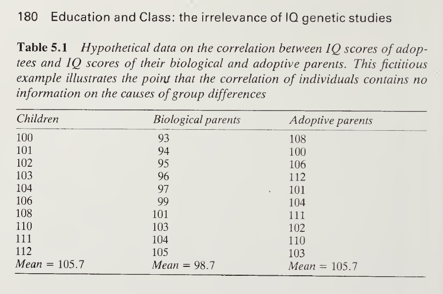
Do we see this pattern in real data? Yes. The most famous illustration comes from Skodak and Skeels (1949), who followed 100 children born to low-IQ biological mothers (mean IQ approximately 86) and adopted into enriched homes. The following is from Templeton’s textbook (Human Population Genetics and Genomics) describing the study:
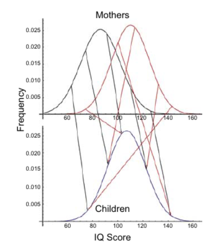

Some notes on the Skodak and Skeels data are in order. Later analyses found that the original biological-mother IQ estimates were somewhat too low (problems with the test norms used), and that Flynn Effect corrections reduce the apparent gain. After these corrections, the best estimate of the adoption gain is approximately 13 points rather than the originally reported 20+ [Flynn 1993, Intelligence]. The children’s mean IQ also appeared to decline from approximately 117 at age 2 to approximately 108 by age 13 on the 1916 Stanford-Binet [Kendler et al. 2015, citing S&S data]. Most of this apparent decline is a test artifact rather than a real cognitive change, however. The age-2 scores were based on the Kuhlmann-Binet—a different instrument whose items at that age are heavily weighted toward sensorimotor and early-language tasks, and which has low predictive validity for later IQ [Skodak & Skeels 1949, p. 93]. Moreover, the 1916 Stanford-Binet produces progressively lower scores at older ages relative to other IQ tests: the Terman-Merrill equivalence table shows the 1916 and 1937 Stanford-Binet give nearly identical scores at ages 5–11 but the 1916 scores fall progressively below from ages 12 to 18 [Flynn 1993, citing Terman & Merrill 1937, p. 50]. Skodak and Skeels recognized this problem independently. At the final follow-up (age 13), they administered both the 1916 Stanford-Binet and the 1937 Stanford-Binet Form L simultaneously to all 100 children. On the 1916 test, the mean IQ was 107; on the 1937 Form L, it was 117—a 10-point discrepancy on the same children on the same day [Skodak & Skeels 1949, Table 4]. The two tests correlated at .92, confirming they ranked the children identically; the difference was entirely in absolute level. The age-by-age data make the pattern vivid: at age 10 the two tests gave identical means, but by age 14 the 1916 test scored 11 points lower than the 1937 Form L [Skodak & Skeels 1949, Table 5].64 What matters is the final, corrected measurement. Even using Flynn’s conservative estimate based on the 1916 test alone, the adopted children at age 13 scored approximately 106–110—still roughly 13 points above their biological mothers after corrections, and close to the adoptive-family mean [Flynn 1993]. The gain did not fade away. It stabilized at a level well above what would have been expected without adoption.
This pattern—correlations tracking biological parents while the group mean tracks the adoptive environment—was replicated in the Texas Adoption Project [Horn, Loehlin, & Willerman 1979; described in Cognitive Development of Adopted and Fostered Children, Turkheimer 1986]. Turkheimer’s dissertation reviewed many adoption studies up to that time and noted that most tracked the correlations rather than taking data that allowed checking how close the group means were to the adoptive family. Even without that direct comparison, however, the studies consistently showed that adoption had a significant effect on group mean IQ relative to the relevant reference groups.
These patterns—the correlation pattern and the significant effect on mean IQ—have been confirmed in adoption studies involving black adoptees as well, as we will see below.
Why do the adoptive-parent correlations decline? The hereditarian reads the declining correlations with adoptive family members as evidence that the shared family environment ceases to matter. But Burt et al. (2024, Behavior Genetics) [verify full citation: this appears to be from Springer] offered a more precise explanation. They showed that low adoptive-parent–adoptee correlations are substantially explained by measurement noise in the shared-environment component. As children age, the signal-to-noise ratio for detecting shared environmental effects worsens—not because the environment stopped mattering, but because the statistical methods used to partition variance have difficulty separating shared environment from error at later ages. The mean IQ of adopted children remains elevated—the environment demonstrably did something—but the correlation-based methods that behavioral geneticists use to detect shared environment lose power. Burt’s finding matters because it removes the last pillar of the “correlation proves genetics won” argument: the declining correlations are not even clean evidence that shared environment effects diminish; they may be substantially a measurement artifact.
We see, then, that the correlations are a distraction—irrelevant in principle (Lewontin’s point), not reflective of reality in the data (Skodak & Skeels, Texas Adoption Project), and not even measuring what hereditarians think they measure (Burt). What matters is the absolute gain from adoption. How large is that gain, and does it persist?
3.10.2 What General Adoption Studies Show
The most methodologically rigorous modern adoption study is Kendler et al. (2015, PNAS), which used Swedish national registries to study siblings reared together versus adopted apart—a design that holds genetics constant within sibling pairs while varying the environment. The sample was large (over 600 male sibling pairs with cognitive data), and the design avoids the self-selection problems that plague smaller studies. Kendler found a clear dose-response relationship: the larger the gap in environmental quality between the biological and adoptive homes, the larger the IQ gain from adoption. Adoptees raised in the most enriched homes gained substantially compared to their non-adopted siblings; adoptees raised in homes similar to their biological families gained little. This is precisely what one expects if environmental quality causally affects IQ, and it is difficult to explain under any model in which IQ is fixed at conception. Kendler’s findings also help explain the Skodak and Skeels results: the smaller gains after correction (approximately 13 points rather than 20) are consistent with the biological homes not being as deprived, or the adoptive homes not being as enriched, as originally estimated.
Across the adoption literature more broadly, the pattern is consistent: adoption into enriched homes produces IQ gains of approximately 10–15 points relative to non-adopted siblings or to the biological-parent mean, with the size of the gain depending on the magnitude of the environmental change [Capron & Duyme 1989; van IJzendoorn, Juffer, & Poelhuis 2005 meta-analysis; Kendler et al. 2015] [verify Capron & Duyme and van IJzendoorn figures]. In the most dramatic demonstration, Duyme, Dumaret, and Tomkiewicz (1999, PNAS) followed 65 French children adopted at ages 4–6 from abusive or neglectful backgrounds (mean IQ approximately 77 at adoption). By ages 13–18, their IQ had increased by 7.5 to 19.5 points depending on the SES of the adoptive family—with children adopted into high-SES families gaining the most [verify exact figures from Duyme et al. 1999].
Do the gains persist? By “fadeout” here we mean the hereditarian’s specific claim: that adoption gains are temporary, and that adopted children’s IQ eventually returns to the level predicted by their biological parents as genetic influences reassert themselves with age. This is the claim that matters for the race debate—that the IQ gap is genetically fixed and cannot be permanently moved by environmental change. We should distinguish this from the more modest possibility that adoption gains attenuate somewhat from childhood peaks without disappearing. Some attenuation would not be surprising—a child tested at age 4 in a novel, stimulating environment may score at an unsustainably high peak—and would not vindicate the hereditarian position so long as the gains remain substantial.
No adoption study has demonstrated that IQ gains from adoption fade back to biological-parent levels. Skodak and Skeels showed some apparent decline from early peaks, but as we saw, most of that decline is a test artifact, and the gain at age 13 remained substantial under every correction. The Minnesota Transracial Adoption Study (discussed in detail below) showed IQ decline for every group at follow-up—including the adoptive parents and their biological children—which the authors attributed to using different IQ tests at the two time points, not to fadeout from adoption. In every case where the adoption gain could be measured against biological-parent IQ, it persisted. Duyme, Dumaret, and Tomkiewicz (1999) provided particularly strong evidence: their sample of 65 French children had been adopted at ages 4–6 from abusive or neglectful backgrounds, meaning the pre-adoption IQ (approximately 77) was measured, not estimated from parental proxies. At ages 13–18, the gains of 7.5 to 19.5 points were fully intact—measured 7 to 12 years after adoption, well into adolescence. The gains did not fade.
More recently, Willoughby et al. (2021, Behavior Genetics) provided the strongest evidence for long-term persistence. In a large adoption study (adopted children were 21% white, 66% Asian, and 13% “other ethnicities”), IQ was measured at age 15 and again at age 30—well past the point at which hereditarians claim genetic influences should have fully asserted themselves. The results:
| Adopted | Biological | Cohen’s d | |
|---|---|---|---|
| Total IQ (age 15) | 106.6 | 108.07 | 0.11 |
| Verbal IQ (age 15) | 101.94 | 103.75 | 0.13 |
| Vocabulary (age 15) | 10.38 | 10.62 | 0.1 |
| Vocabulary (age 30) | 10.79 | 10.88 | 0.04 |
| ICAR-16 (age 30) | 8.87 | 9.93 | 0.28 |
Table: Relevant data from Willoughby et al. (2021). Cohen’s d measures the difference between groups in standard deviation units; values below 0.2 are conventionally considered negligible (see our earlier discussion of effect sizes).
Two things stand out. First, the vocabulary scores—which hereditarians consider the most g-loaded and the most correlated with innate intelligence—were essentially identical for adopted and biological children at both ages, with the already-trivial gap shrinking from d = 0.10 to d = 0.04 over fifteen years. Second, the ICAR-16 at age 30 showed a modestly larger gap (d = 0.28), but this was a different and much shorter test than the one administered at age 15 (16 items versus a full IQ battery), making direct comparison difficult. As we saw with Skodak and Skeels—where two IQ tests given on the same day to the same children produced means 10 points apart—switching instruments can easily produce apparent changes that are artifacts of the test rather than real cognitive shifts. The vocabulary data, which use the same subtest at both ages and therefore avoid this problem, provide the cleanest evidence: adoption’s effects on crystallized intelligence do not fade even well into adulthood. The ICAR-16 result could reflect genuine partial attenuation of fluid intelligence gains, or it could reflect the inherent difficulty of comparing scores across different instruments; the data do not allow us to distinguish these possibilities.
An important caveat: Willoughby did not report biological-parent IQ for the adoptees, so we cannot directly calculate the magnitude of the adoption gain—only that the gap between adopted and biological children did not grow from age 15 to 30. This is a common limitation of adoption studies; Turkheimer (1986) noted that few studies collect the data needed to compare adopted children’s IQ to what would have been expected without adoption. Studies that do allow this comparison—Skodak and Skeels, the Texas Adoption Project, and Kendler—consistently show substantial gains.
Summary. The general adoption literature establishes several facts. Adoption into enriched homes raises IQ, with the gain proportional to the magnitude of the environmental change (Kendler). The gains are substantial—on the order of 10–15 IQ points in the strongest designs. No study has demonstrated complete fadeout of adoption gains back to biological-parent levels. The best long-term evidence (Willoughby) shows no fadeout of vocabulary scores from age 15 to 30; whether there is modest attenuation of fluid intelligence gains is uncertain, because the only relevant measure used a different and much shorter test. Apparent declines in older studies (Skodak & Skeels, MTAS) are substantially attributable to test-change artifacts rather than genuine cognitive fadeout. The mechanism is real, replicable, and of sufficient magnitude that it could, in principle, explain most or all of a 10–15 point group difference. Whether it actually does so for the racial IQ gap is the question the transracial studies address.
3.10.3 Transracial Adoption Studies
We now turn to the direct evidence: studies in which children of black or part-black ancestry were raised by white families and tested for IQ. These studies are few, small, and imperfect. But they are the closest thing we have to a direct experimental test of whether the black-white IQ gap survives when the environment is equalized. We will go through them one by one, as Thomas (2017, Journal of Intelligence) does, beginning with the earliest and ending with the Minnesota Transracial Adoption Study—the one hereditarians rely on most heavily.
Eyferth (1961). After World War II, children fathered by American occupation soldiers and German women were raised in Germany by their mothers or in German institutions. Eyferth tested these children at school age. The key comparison: children fathered by white American soldiers versus children fathered by black American soldiers. Because the mothers were all German, the groups differed in paternal race but shared the same maternal population and the same rearing environment. The children were biracial in both cases (half American, half German), so the hereditarian prediction is that the black-fathered children should score approximately half a standard deviation (about 7–8 points) below the white-fathered children, reflecting the genetic contribution of the black fathers.
Eyferth found no significant IQ difference between the groups. The black-fathered and white-fathered children scored essentially the same—approximately 96–97 for both groups [Eyferth 1961; N approximately 181 white-fathered, 83 black-fathered; verify exact Ns against primary source]. A 95% confidence interval for the difference, assuming SD = 15, is approximately -3 to +5 points. A deficit of 7–8 points—the hereditarian prediction—is excluded at conventional significance levels [at (-7.5 - 0.7)/1.99 ≈ -4.1 standard errors, p < 0.001].
The hereditarian raises several objections [Rushton & Jensen 2005]. First, that black American soldiers were screened by Army cognitive tests and therefore more cognitively selected than white soldiers. This is true to a degree, but white soldiers were screened by the same tests. The question is whether the screening was differentially selective, and while it was—the lower black population mean means a larger fraction was screened out—the screening cutoff was not stringent enough to produce 7–8 IQ points of differential selection [Flynn 1980]. Moreover, the hereditarian’s own framework predicts that differential screening cannot close the gap. Even if the black soldiers who passed the screening had IQs comparable to their white counterparts, the hereditarian model holds that their children should regress toward the lower black genetic mean, while the white soldiers’ children regress toward the higher white genetic mean. On the hereditarian’s own account, screening can narrow the gap between the fathers but cannot prevent the gap from reappearing in the children. The null result contradicts not just the simple hereditarian prediction but the prediction as modified by the hereditarian’s own regression model.65
Second, that the children were tested young. We have addressed this objection: heritability is already approximately 0.40–0.45 at school age [Plomin & Deary 2015], and if a large genetic effect existed, it should be detectable when heritability is already substantial.
Third, that some “black” fathers may have been North African rather than sub-Saharan African. Eyferth sampled from both the American and French occupation zones (Eyferth 1959, p. 105), and approximately 20–25% of the colored children’s fathers served in French rather than American forces—a figure originating in Eyferth, Brandt, and Hawel (1960, p. 13) and independently confirmed by Flynn’s geographic analysis of the sample (Flynn 1980, p. 85). Rushton and Jensen (2005) cite this figure but recharacterize these fathers as “French North Africans (i.e., largely Caucasian or ‘Whites’ as we have defined the terms here).” This is another instance of Rushton and Jensen presenting an unsupported inference as established fact: no source they cite describes these fathers as Caucasian, and the characterization is contradicted by both Flynn’s terminology and Eyferth’s own classification of his subjects.66
Even granting the claim, the arithmetic does not rescue the hereditarian prediction. The “black”-fathered group averaged approximately 97. If 25% of that group (roughly 43 of 170 children) were North African-fathered, the remaining sub-Saharan subgroup (n ≈ 127) would need to average approximately 89.5 to produce the predicted 7–8 point gap with the white-fathered group. For that to happen, the North African-fathered children would need to have averaged approximately 119—twenty-two points above the white-fathered biracial children, well into the gifted range. No one claims North African populations outscore Europeans by that margin; on the hereditarian’s own data they score below Europeans. Even in a generous scenario where the North African-fathered children scored 105, the sub-Saharan subgroup mean drops only to about 94, producing a gap of roughly 3 points—less than half the hereditarian prediction and within sampling noise. Flynn (1980, p. 90) performed a similar calculation and concluded that even under the most favorable assumptions, the non-American fathers could shift the overall colored mean by less than one point.
Fourth, there is a sex × race interaction in the data: white-fathered boys scored notably higher than white-fathered girls—an unusually large sex difference suggesting sampling error—while the sex difference among black-fathered children was negligible [Loehlin 2000]. Flynn (1980) analyzed this interaction at length and concluded it did not undermine the overall null finding [verify against Flynn 1980, chapter on Eyferth]. We note it for transparency; the overall comparison, averaging across both sexes, remains the more reliable estimate, and Kirkegaard’s independent replication (below) found no gap either.
Kirkegaard, Lasker, and Kura (2019) replicated Eyferth’s finding using data from biracial children of U.S. servicemen and Japanese women in post-war Japan, again finding no IQ difference by father’s race [Kirkegaard et al. 2019, Psych]. This replication is notable because Kirkegaard is a hereditarian researcher; the finding is a concession from the hereditarian side. The environmental model predicts these results. The genetic model is contradicted unless one posits ad hoc assumptions about differential selection that exactly compensate for the supposed genetic disadvantage.
Tizard (1974). In British long-stay residential nurseries, where all children received the same institutional care from the same staff, Tizard tested black, white, and mixed-race children at approximately age 4.5. The black children were of West Indian (Caribbean immigrant) parentage. The hereditarian might object that immigrants are positively selected, inflating the black children’s IQ. This concern is real but limited: Flynn estimated that cognitive selection effects for West Indian immigrants to Britain could not have raised the parental IQ by more than a few points (Flynn 1980, cited in Nisbett 1998, p. 96 [verify page]), and the symmetry argument applies—the white children in these nurseries were also not a random draw from the general population but children whose families placed them in institutional care, a circumstance associated with social disadvantage. Neither group’s parents are representative, and the biases run in opposite directions. The environment in the nursery was essentially uniform—the nursery, not the children’s biological families, determined the rearing conditions.
The results: no significant IQ differences between groups. Using the means reported in the original study [verify against Tizard 1974, Nature; there is a discrepancy between Nisbett’s reported means (black ≈ 108, white ≈ 103) and other sources (black ≈ 105.6, white ≈ 106.0)—trace to primary source before publication], the black children scored at or slightly above the white children.
The sample is small (approximately 9 black, 36 white, 19 mixed-race in the full nursery sample), and hereditarians dismiss it on this basis. But even at n = 9, the confidence interval is informative. Using a conservative SD of 10 and the more conservative set of means (approximately equal), the 95% CI for the black-white difference is approximately ±7 points. A deficit of 15 points—what the strong hereditarian model predicts for fully black children in a shared environment—falls nearly 4 standard errors below the observed difference and is firmly excluded (p < 0.001). Tizard cannot establish a precise environmentalist result, but it rules out what the strong hereditarian thesis requires. Small samples can exclude large effects.
Willerman, Naylor, and Myrianthopoulos (1974). This study examined 129 biracial (black-white) 4-year-olds—a substantially larger sample than Moore or Tizard. The key finding: biracial children with white mothers scored approximately 9 points higher (mean IQ 102) than biracial children with black mothers (mean IQ 93). The gap was not explained by SES—the groups had similar socioeconomic backgrounds—and it persisted after controlling for marital status.
This finding is difficult for the genetic model. Both groups of children have the same racial mixture (half black, half white), so genetics predicts they should score the same. The variable that differs is which parent is white and which is black—and therefore which parent’s environment (prenatal, perinatal, and early postnatal) the child experienced. Children who gestated in a white mother’s body and spent their early months in a white mother’s household scored a full 9 points higher than children who gestated in a black mother’s body and spent their early months in a black mother’s household. The genetic composition is held constant; the environment differs; the IQ differs. This is what the environmental model predicts.
The hereditarian will object that the white and black mothers may have differed in IQ, not just in the environment they provided—making the results “not interpretable” without equal mid-parent IQs [Rushton & Jensen 2005, citing Loehlin et al. 1975]. But the SES differences between the groups were trivially small. Maternal education differed by less than one year (11.3 vs. 10.5), as did paternal education (11.5 vs. 10.7). The Bureau of Census socioeconomic index—a composite measure incorporating occupation—was nearly identical (46.6 vs. 44.6 on a scale with SD ≈ 20). Family income actually favored the black-mother group ($3,888 vs. $3,469). Birth weight, birth length, gestational age, and number of prior children were likewise indistinguishable. None of these differences approached statistical significance [Willerman et al. 1974, Table I]. Willerman et al. themselves concluded that if genetic selection had produced a meaningful IQ advantage in one mating type over the other, “one would expect that this superiority should have been detectable in the educational, socioeconomic, or income levels reported in Table I. That such differences were not observed places in doubt such a contention.” These near-identical SES profiles constrain how large any IQ difference between the mothers could plausibly be. Even granting a moderate maternal IQ difference—say, 5 points—the expected effect on the children’s IQ via genetic transmission alone would be roughly 1–2 points (half the maternal contribution, attenuated by heritability), far short of the approximately 9-point gap observed. The gap is too large to attribute to plausible differences in maternal IQ.
A caveat: white and black mothers of biracial children in the 1970s differed in many ways beyond race—cultural context, social network, the particular circumstances that led to an interracial relationship at that time. The finding is suggestive of a maternal-environment effect, not a decisive proof. But it is consistent with and adds to the pattern we will see in Moore.
Moore (1986). Moore studied 46 black-ancestry children adopted into either white families (n = 23) or black families (n = 23). The aggregate result: children in white homes scored approximately 117, children in black homes approximately 104—a 13.5-point gap attributable to the adoptive family environment [Thomas 2017, Table 1].
The hereditarian will object that the two groups were not racially identical: the white-home group included more biracial children and the black-home group included more fully black children, because black adoptive parents disproportionately requested children resembling them [Moore acknowledged this confound; Warne 2023, “Revisiting Moore’s transracial adoption study,” provides the breakdown]. The sample breaks down as follows:
| Group | Fully Black | Biracial (B-W) | Total |
|---|---|---|---|
| White adoptive families | 9 | 14 | 23 |
| Black adoptive families | 17 | 6 | 23 |
[Source: Warne 2023; Thomas 2017 Table 1 for means and SDs]
This confound can be addressed in two steps. First, compare the fully black children across family types, removing the confound entirely: fully black children in white homes (n = 9, mean IQ = 118.0, SD = 10.5) versus fully black children in black homes (n = 17, mean ≈ 103) [verify black-home fully-black mean; approximately 103 from the aggregate data]. The gap is approximately 15 points—even larger than the aggregate comparison, not smaller. The 95% confidence interval for this difference, assuming similar SDs for both groups, is approximately 6.5 to 23.5 points [SE ≈ 4.4, CI = 15 ± 8.6]. The entire confidence interval is above zero; this effect is statistically significant even at n = 9 versus n = 17, because the effect is large.
Second, within the white-home group, compare the fully black and biracial children: fully black in white homes scored 118.0, biracial in white homes scored 116.5 [Thomas 2017, Table 1]—a trivial 1.5-point difference, in the wrong direction for the hereditarian (the fully black children scored slightly higher). Within the black-home group, the pattern is similar: biracial children scored 105.7, fully black children 102.9—a small difference, and plausibly attributable to the non-random placement confound or to chance at these small sample sizes.
The two-step argument: removing the confound did not shrink or reverse the effect of adoptive-family race; if anything, it grew larger. This means the aggregate 23-vs.-23 comparison is valid—the confound was not driving the result. The adoptive family’s race matters more than the child’s degree of African ancestry.
A hereditarian might set aside the within-group comparisons and note that collapsing across family type, biracial children in the aggregate scored 5.1 points higher than fully black children (one-tailed p = .037) [Warne 2023]. But this aggregate comparison is confounded by the very placement pattern described above. Biracial children were concentrated in white homes (14 of 20, or 70%), while fully black children were concentrated in black homes (17 of 26, or 65%). If placement had been equal—50% of each ancestry group in each family type—the expected means would be approximately 111.1 for biracial children and 110.5 for fully black children, a difference of about half a point.67 Approximately 88% of the aggregate 5.1-point “hereditarian finding” is an artifact of the environmental confound. This is why within-group comparisons, not collapsed aggregates, are the appropriate test.
Moore also observed a qualitative difference in parenting practices. During problem-solving tasks administered as part of the study, middle-class black adoptive mothers were “much more reprimanding and scornful” while middle-class white mothers were “much more encouraging and rewarding” [Moore 1986]. This suggests a mechanism: differences in parenting style, independent of socioeconomic status, that affect cognitive development. The mechanism is environmental.
Honest limitation: non-random placement is a confound that the two-step argument reduces but does not eliminate entirely. Children placed with white families may have differed from children placed with black families in ways beyond the fully-black/biracial distinction—health at placement, pre-adoption experiences, agency decisions we cannot observe. Moore is suggestive and powerful, but not conclusive on its own.
The Minnesota Transracial Adoption Study (MTAS). - AI gen This is the study hereditarians cite most often, because they believe it supports their position. Scarr and Weinberg (1976) initially reported on 101 families who had adopted black, biracial, and white children. The children were tested at approximately age 7 (Time 1). Weinberg, Scarr, and Waldman (1992) published a follow-up when the children were approximately 17 (Time 2). Because this is the hereditarian’s preferred study, we will examine it in detail.
At Time 1, all adopted groups scored well above the regional black average of approximately 90 for the North Central region [Scarr & Weinberg 1976, p. 736, citing Kaufman & Doppelt]—evidence that adoption into enriched white homes raised IQ for every group. At Time 2, IQ had declined for every group, including the adoptive parents and their biological children. The following table gives the mean IQ scores across the three time points. “Time 1b” is the subset of participants who were present at both Time 1 and Time 2—the matched cohort whose scores can be compared directly across ages without attrition contamination. “Time 2 (corrected)” applies Thomas’s (2017) correction for differential attrition, described below.
| Time 1a | Time 1b | Time 2 | Time 2 (corrected) | |
|---|---|---|---|---|
| Fathers | 120.8 | 121.7 | 117.1 | — |
| Mothers | 118.2 | 119.1 | 113.6 | — |
| Biological Offspring | 116.7 | 116.4 | 109.4 | — |
| Black/Black Adopted | 96.8 | 95.4 | 89.4 | 90.1 |
| Black/White (Biracial) Adopted | 109.0 | 109.5 | 98.5 | 98.3 |
| All Socially Black/Interracial Adopted | 106.3 | 106.1 | 96.8 | ~96.9 |
| White Adopted | 111.5 | 117.6 | 105.6 | 101.8 |
| Black/Black–White Gap | 14.7 | 22.2 | 16.2 | 11.7 |
Sources: Time 1a, Time 1b, and Time 2 values from Weinberg, Scarr, & Waldman 1992, Table 2. Time 2 (corrected) values from Thomas 2017 (combined B/I value is our computation applying Thomas’s method to the combined group). The “All Socially Black/Interracial” row is the study’s original analytical unit: all 130 children socially classified as black, including 68 biracial (black/white), 29 fully black, and 33 with other interracial or unspecified parentage [Scarr & Weinberg 1976]. This combined group is useful for the study’s broad question—whether socially black children raised in white homes kept pace with white adoptees over time—though it is not useful for testing the hereditarian admixture prediction, since it combines children of different ancestry proportions.
The sample sizes, ranges, and standard deviations underlying these means matter for interpretation and are given in the following table [Weinberg, Scarr, & Waldman 1992, Table 2]:
| Time 1a | Time 1b | Time 2 | |
|---|---|---|---|
| Black/Black | n=29, SD=12.8, range 80–130 | n=21, SD=13.3, range 80–130 | n=21, SD=11.7, range 75–112 |
| Biracial | n=68, SD=11.5, range 86–136 | n=55, SD=11.9, range 86–136 | n=55, SD=10.6, range 73–134 |
| All B/I | n=130, SD=13.9, range 68–144 | n=101, SD=14.7, range 68–144 | n=101, SD=12.0, range 71–134 |
| White | n=25, SD=16.1, range 62–143 | n=16, SD=11.3, range 92–138 | n=16, SD=14.9, range 79–140 |
| Bio Offspring | n=143, SD=14.0, range 81–150 | n=104, SD=13.5, range 86–150 | n=104, SD=13.5, range 78–146 |
Two features of this table should be noted. First, the follow-up white-adoptee group is very small: n=16. This is the comparison group on which the hereditarian interpretation rests. Second, the white group’s Time 1 range compressed dramatically from Time 1a (62–143) to Time 1b (92–138). The lowest-scoring white adoptees dropped out of the study. This attrition did not merely reduce the sample; it changed who was being compared, as we will see below.
The hereditarian reads this table as showing a widening gap: the raw black/black–white difference went from 14.7 points at Time 1a to 16.2 points at Time 2. But this reading does not survive scrutiny.
The hereditarian prediction of widening fails. The correct way to measure gap trajectory is to compare the same individuals at both time points. The Time 1b cohort—those who returned for the follow-up—had a black/black–white gap of 22.2 points. At Time 2, the same individuals showed a gap of 16.2 points. The gap narrowed by 6.0 points in the matched individuals. The authors confirmed: “There were no adopted group differences in IQ decline” [Weinberg, Scarr, & Waldman 1992, p. 124].68 Two caveats are needed. First, the returning white cohort was positively selected by attrition (Time 1b mean of 117.6 versus Time 1a mean of 111.5), so the 22.2-point starting gap is inflated—the matched comparison is already biased against finding narrowing. Second, while the point estimate favors narrowing, a difference-in-differences test of the decline rates between the black/black and white groups does not reach statistical significance (approximate t ≈ 1.5, p ≈ .15; our calculation from Table 2 standard deviations and Time 1–Time 2 correlations). This is unsurprising at n = 21 and n = 16. The study lacks the power to detect moderate trajectory differences in either direction. What it does have the power to show is that the large, decisive widening predicted by Rushton and Jensen—who had specifically predicted that “Trait differences not apparent early in life begin to appear at puberty and are completely apparent by age 17” (p. 259)—did not occur.69
Every group declined, for reasons unrelated to genetics. The adoptive parents’ IQ dropped by 3–5 points. The biological children dropped by 7 points. This universal decline was attributed by the authors to using different IQ tests at the two time points (Stanford-Binet at Time 1 versus WISC-R/WAIS-R at Time 2). A decline that affects every person in the study—including adults whose IQ should be stable—is a measurement artifact, not a genetic process asserting itself.
Differential attrition inflated the white group at Time 2. Not all participants returned for the follow-up. The white group was hit hardest: 9 of 25 white adoptees dropped out, and as the detail table above shows, those who dropped out were the lower-scoring members of the group. The returning white group’s Time 1 mean was 117.6, compared to the original white mean of 111.5—a 6.1-point inflation. The black/black group showed a much smaller attrition effect (Time 1b mean of 95.4 versus original 96.8, a shift of only 1.4 points). This asymmetry means that the Time 1b–to–Time 2 comparison, where the gap narrowed by 6.0 raw points, is already biased against finding narrowing: it compares a selectively higher-scoring white group against a roughly representative black group.
Thomas (2017, Journal of Intelligence) corrected for this attrition by adjusting the Time 2 scores to reflect the original, unselected groups. After correction, the Time 2 scores become: Black/Black = 90.1, Biracial = 98.3, White = 101.8. The corrected black/black–white gap is 11.7 points—smaller than the Time 1a gap of 14.7 points. Thomas’s correction confirms from a different angle what the matched-individual comparison already showed: the point estimate favors narrowing, and the predicted widening did not occur.
We broadly agree with Thomas’s assessment: the MTAS data, while inconclusive on its own, does not support the hereditarian hypothesis. The widening claim is the study’s most directly testable prediction, and it fails under every known correction. Where we extend Thomas’s analysis is in examining the Flynn effect directly.
The Flynn effect does not reverse this result. Thomas (2017) noted a complication: because the children took different IQ tests depending on age at Time 1 (younger children took the Stanford-Binet, older children took the WISC), and because the black children were younger on average than the white children, the two groups were differentially affected by the Flynn effect—the tendency for IQ scores to be inflated by outdated test norms. Thomas acknowledged this “could conceivably eliminate the attrition effect while restoring the widening of racial IQ gaps over time, but there is little a priori reason to expect that.” Thomas referred to Loehlin (2000), who reported MTAS means adjusted for “norm shifts over time,” but described the data as “too meagre to permit detailed analysis.” Loehlin’s corrected values were based on data from the original investigators [Waldman, Weinberg & Scarr 1996, unpublished conference presentation at the International Society for the Study of Behavioral Development, Quebec City]. The correction method is not documented and the source is unpublished, so the values should be treated cautiously—we cannot vouch for their accuracy given so many unknowns. Loehlin’s n values (21, 55, 16) match the Time 2 returning sample sizes, confirming that his “Original Study” values are the Flynn-corrected Time 1b means—the returning cohort, not the full original sample.70 Even Loehlin’s Flynn-corrected data shows the black/black–white gap narrowing in the matched individuals:
| Loehlin Time 1b | Loehlin Time 2 | Decline | n | |
|---|---|---|---|---|
| Black/Black | 91.4 | 83.7 | −7.7 | 21 |
| Biracial | 105.4 | 93.2 | −12.2 | 55 |
| White | 111.5 | 101.5 | −10.0 | 16 |
| Asian/Indian | 96.1 | 91.2 | −4.9 | 12 |
| Bio Offspring | 110.5 | 105.5 | −5.0 | 101 |
The matched comparison (same individuals at both time points, Flynn-corrected) is the cleanest result Loehlin’s data provides. The black/black–white gap narrows from 20.1 to 17.8 (−2.3 points), and the Asian/Indian–white gap narrows from 15.4 to 10.3 (−5.1 points). The biracial–white gap widens slightly (6.1 → 8.3, +2.2 points), consistent with the small fluctuations in both directions seen under other methods. None of these changes is statistically significant at n = 16 whites.
This matched comparison does not depend on attrition correction: it tracks the same people over time. A proper attrition correction on Loehlin’s Flynn-corrected data cannot be precisely computed because Loehlin does not provide his corrected Time 1a values, and the published age distributions do not break out subgroups (see note).71 What we can say is directional: attrition inflated the white group’s scores by far more than any other group (6.1 points versus 1.4 or less), so the Time 2 gap under Loehlin is larger than the true full-population gap. Applying Thomas’s raw-data attrition adjustments as a rough approximation suggests the B/B–white Time 2 gap drops to approximately 13.3 and the biracial–white gap to approximately 4.7—but these are indicative of the direction attrition correction pushes, not precise estimates. The approximation mixes populations across time points (the Time 1b starting gap is itself attrition-inflated, while the Time 2+att endpoint is de-attrited), which overstates the narrowing relative to a properly de-attrited comparison at both time points. For the B/B–white gap, the overstatement is substantial enough (~4.5 points) that the true full-population trajectory under both Flynn and attrition correction could range from slight narrowing to approximate stability—we cannot determine which without individual-level data. What we can exclude is the predicted substantial widening: even in the least favorable calculation, the B/B–white gap trajectory falls within roughly ±2 points of stable. The approximate attrition correction thus provides evidence for Thomas’s assessment that there is “little a priori reason to expect” Flynn correction would produce widening, without our needing to commit to a specific corrected value.
An approximate significance test of the matched B/B–white narrowing—using the raw standard deviations, which are only a rough proxy because the Flynn correction varies by individual depending on which test each child took at Time 1—yields t ≈ 0.6, p ≈ .57: far from significance regardless of the exact SDs.
This study does not provide clean evidence that adoption gains faded; the universal declines are primarily test artifacts, as discussed in a note.72 The authors themselves attributed the declines to the change in test instruments, noting that the documented WAIS-to-WAIS-R co-norming decline of 6.8 points [Sattler 1988] was “precisely the test combination used for adoptive parents in our study” [Weinberg, Scarr, & Waldman 1992, p. 130], and that “substantial declines would be expected” from the Stanford-Binet-to-WISC-R transitions used for the children [citing Flynn 1984]. The Skodak and Skeels data provide the most direct demonstration of this mechanism: two different IQ tests administered to the same children on the same day produced means 10 points apart, with the discrepancy growing systematically with age. When different tests give dramatically different absolute scores to the same individuals, apparent declines across test changes cannot be interpreted as cognitive fadeout. The fadeout question is addressed with stronger evidence in our earlier discussion of the general adoption studies.
The black/black–white gap under every calculated version of the data:
| Version | Time 1 Gap | Time 2 Gap | Change |
|---|---|---|---|
| Raw (Time 1b → Time 2, same individuals) | 22.2 | 16.2 | −6.0 (narrowing) |
| Thomas attrition correction (Time 1a → corrected Time 2) | 14.7 | 11.7 | −3.0 (narrowing) |
| Loehlin Flynn correction (Time 1b → Time 2, same individuals, Flynn-corrected) | 20.1 | 17.8 | −2.3 (narrowing) |
Point estimates favor narrowing under every correction method. However, none of these changes reaches statistical significance at the available sample sizes (n = 21 black/black, n = 16 white). The point-estimate pattern is nevertheless worth noting: hereditarians routinely cite point estimates from this study—particularly the Time 2 level comparisons—without discussing statistical significance, and the same point estimates, applied to the trajectory question, consistently go against the hereditarian prediction. The robust finding is not that narrowing is proven, but that the predicted widening did not occur—and that no version of the black/black–white data that has been computed shows widening. We concede that in theory, a fully correct Flynn and cross-instrument correction—applied with individual-level data and handling the difficult cross-family equating between Stanford-Binet and Wechsler scales—could in principle produce a different result. But the structural asymmetry between the Time 1 and Time 2 test batteries makes this unlikely: the Time 1 norm-staleness spread was large (23 years between the 1949 WISC norms and the 1972 Stanford-Binet norms), while the Time 2 spread was small (7 years between the 1974 WISC-R norms and the 1981 WAIS-R norms). Any correction that shrinks the Time 1 gap more than the Time 2 gap—which the structural asymmetry strongly favors—produces narrowing. Every correction that has actually been computed confirms this direction for the black/black–white comparison. The burden of proof is on anyone claiming an uncalculated correction would reverse what every known correction shows.
The biracial-white comparison is ambiguous. At Time 1, the biracial–white gap was only 2.5 points (SE = 3.5; Thomas 2017)—already not significantly different from zero. After Thomas’s attrition correction at Time 2, the gap is approximately 3.5 points. With a Flynn/norm correction layered on, the estimate rises to approximately 4.2–4.7 points. The gap did not meaningfully change from Time 1 to Time 2, and it was never large enough to reach statistical significance. The expected hereditarian gap depends on the baseline: under the national 15-point black-white gap, a simple midpoint prediction gives ~7.5 points; under a regional baseline closer to 10–12 points—Scarr and Weinberg themselves noted that “the average IQ of 90 [is] usually achieved by black children reared in their own homes in the North Central region” [Scarr & Weinberg 1976, p. 736, citing Kaufman & Doppelt]—the expected hereditarian gap is only ~5–6 points. (The “90” here refers to all socially classified black children in the North Central region, not only fully black children.) The observed estimate falls at the low end of the hereditarian-compatible range. At n=16 and n=55, the confidence intervals include both the environmental prediction of approximately zero and the hereditarian prediction of approximately 5–6 points. This comparison cannot bear decisive evidential weight for either side.
The combined socially-black/interracial group provides a more precisely estimated comparison. This group—all 101 children who would have been classified as “black” in American society, regardless of exact parentage—scored 96.8 at Time 2 (SE approximately 1.2), well above both the national black average of approximately 85 and the regional black average of approximately 90. In the raw matched data, the gap between this combined group and white adoptees moved from approximately 11.5 at Time 1b to 8.8 at Time 2, and to approximately 4.9 after attrition correction—consistent with the pattern of no widening seen in the black/black–white data, though the combined group is not useful for testing the hereditarian admixture prediction since it merges children of different ancestry proportions. Even in the hereditarian’s preferred study, adoption substantially raised the IQ of socially black children above the non-adopted black average—a fact that the focus on subgroup differences tends to obscure.
Scarr’s (1998) later assessment. Scarr later wrote that the results were ambiguous and that the investigators “should have been agnostic on the conclusions” [Scarr 1998, Intelligence 26(3), DOI: 10.1016/S0160-2896(99)80005-1 [verify exact title and page numbers]]. The formal published position of all three authors remains that “results from the Minnesota Transracial Adoption Study provide little or no conclusive evidence for genetic influences underlying racial differences in intelligence and achievement” [Waldman, Weinberg, & Scarr 1994, Intelligence 19(1), DOI: 10.1016/0160-2896(94)90051-5 [verify exact page numbers]]. We agree with Scarr that the level comparisons are ambiguous, as the analysis above demonstrates. Where the data speak clearly, however, is on the trajectory: no version of the data produces the widening that hereditarians claim. A study can be “ambiguous overall” while contradicting a specific prediction. “Agnostic” is not “supports the hereditarian reading.”
The MTAS had a late-adoption confound that worked against the environmental model. The combined black/interracial adoptees were placed at a mean age of 18.0 months, nearly identical to the white adoptees’ mean of 19.0 months [Scarr & Weinberg 1976, Table 5]. However, the subgroups differed markedly: fully black children were placed at approximately 32 months on average, biracial children at approximately 9 months, and white children at approximately 19 months [Scarr & Weinberg 1976, Table 10; cf. Loehlin 2000]. The late-placement confound works against the environmental model specifically for the black/black subgroup, which was placed on average 13 months later than white adoptees. This same subgroup also had the most and poorest preadoptive placements and the lowest biological-parent education levels. The biracial children, by contrast, were placed 10 months earlier than whites. We know from the broader adoption literature—and from the MTAS data itself—that earlier placement produces larger gains. In the 1992 follow-up, the early-placed black/interracial children (those placed before their first birthday, n=68 at follow-up) scored 99.2 at Time 2, while the late-placed children (n=33 at follow-up) scored 91.7—a difference of 7.5 points (d = .65, t(99) = 3.06, p = .003) [Weinberg, Scarr, & Waldman 1992]. At Time 1, the gap was even larger: early-placed children scored approximately 11–14 points higher than late-placed children.73 The black/black adoptees were handicapped from the start by late placement. The fact that they still scored at or above the regional black average despite this disadvantage is itself evidence that adoption was working against a headwind.
Achievement scores tell a different story from IQ. Even at age 17, when the raw IQ gaps persisted, the black adoptees scored at the 54th percentile in vocabulary, the 48th percentile in reading, and the 36th percentile in mathematics on standardized achievement tests—well above the non-adopted black average [Weinberg, Scarr, & Waldman 1992]. The vocabulary and reading gaps with white adoptees were less than one-third of a standard deviation (approximately 0.21 SD and 0.25 SD, respectively). These achievement scores are not adjusted for attrition; adjusting would likely reduce the gaps further. Even in the hereditarian’s preferred study, adoption produced real, persistent benefits for black children’s academic performance.
Thomas (2017): Synthesis across studies. Thomas corrected the East Asian adoption studies that hereditarians cite for Flynn effect inflation and for the boost that adoption itself provides (adoptive families are above-average environments). After correction, the apparent IQ advantage of East Asian adoptees largely disappeared—their high scores were artifacts of outdated test norms and enriched adoptive homes, not evidence of genetic superiority. On the other side, most of the apparent IQ disadvantage of black adoptees disappeared after correcting for attrition in the MTAS. Thomas’s combined inverse-variance-weighted estimate across all studies of biracial adoptees: the gap with white adoptees was 0.4 ± 3.1 IQ points.74 Thomas concluded that neither the apparent East Asian advantage nor the apparent black disadvantage in transracial adoption studies survived methodological correction. The reader seeking further detail—particularly on the methodological corrections to the Korean and Vietnamese adoption studies—is directed to Thomas (2017, Journal of Intelligence 5(1), 1), which provides a comprehensive treatment of the full transracial adoption literature.
Summary and assessment of the transracial evidence. What did we learn? Let us be honest about the limitations before stating the conclusions.
The studies are small. The total number of black adoptees across all studies is on the order of a hundred. No single study has the statistical power to precisely estimate the gap in a matched environment. This is a genuine limitation.
But a word about asymmetric standards is in order. Hereditarians dismiss Moore (n = 46), Tizard (n = 9 black children), and Eyferth as too small, while citing East Asian adoption studies of comparable or smaller size without the same criticism: Clark and Hanisee (n = 25), Frydman and Lynn (n = 19). The MTAS follow-up—the hereditarian’s preferred study—has only n = 21 black and n = 16 white adoptees at Time 2. If n = 16 is a sufficient basis for hereditarian conclusions, then n = 23 (Moore) and n = 9 (Tizard) are a sufficient basis for challenging them. The hereditarian cannot apply one evidentiary standard to studies that support the genetic model and a different standard to studies that do not.
Moreover, small samples can exclude large effects. Even at n = 9, the confidence intervals for Tizard exclude a black deficit of 15 points. Even at n = 9 versus n = 17, Moore’s effect is statistically significant because the effect size is large. The strong hereditarian thesis predicts deficits of approximately 1 standard deviation. Effects that large are detectable even in small studies. What small samples cannot do is detect effects of 3–5 points. This is relevant and we will return to it.
The hereditarian raises the selection objection: (Verify) that black children placed for adoption are not representative of the black population and may have been selected for higher genetic potential. Three responses. First, the objection applies symmetrically: white adoptees are also non-representative, placed by the same agencies using the same criteria. If selection inflates black adoptee IQ, it inflates white adoptee IQ by a comparable amount, and the gap between the groups is less affected than the absolute levels. Second, in the MTAS specifically, the black biological mothers had relatively low education levels, and many black children were placed late and from unstable pre-adoption circumstances—the selection, to the extent it existed, does not appear to have been strongly upward on cognitive ability. Third, Moore’s data controls for selection within adoptive-family race: fully black children in white homes scored 118, biracial children in white homes scored 116.5. If agencies had selected “better” black children for white homes, we would expect biracial children—who benefit from both selection and European genetic ancestry, per the hereditarian model—to outscore fully black children. They did not. The selection objection does not fit the data.
The white-mother-environment finding. Across Moore and Willerman, a consistent finding emerges: the environment associated with white mothers and white families produces substantially higher IQ in children of black ancestry. In Moore, the gap between white-home and black-home children was approximately 13.5 points. In Willerman, biracial children with white mothers scored 9 points higher than biracial children with black mothers, with genetics held constant. This pattern is what the environmental model predicts: if the black-white IQ gap is substantially caused by environmental differences correlated with race, then changing the environment should change the IQ, and the race of the environment provider should matter more than the race of the child. That is what we observe.
What the studies are consistent and inconsistent with. The strong hereditarian model makes specific predictions: (1) the gap should persist in matched environments, (2) the gap should widen with age as heritability increases, (3) biracial children should score intermediate between the two groups in a pattern tracking their degree of African ancestry, and (4) the adoptive-family environment should have little effect after early childhood. The widening prediction (2) is contradicted by MTAS under every known correction. The biracial-intermediate prediction (3) is not clearly refuted—biracial children do score intermediate—but the point estimate is somewhat closer to the white mean than the hereditarian predicts, and the confidence intervals are too wide to discriminate between the models given the small samples. The adoptive-family environment matters enormously (Moore). Eyferth and Kirkegaard et al. find no gap at all in biracial children raised in the same environment as white children.
The environmental model predicts: (1) adoption into enriched environments should raise IQ, (2) the gap should not widen with age if the environmental difference is removed, (3) the race of the environment should matter more than the race of the child. All three predictions are confirmed.
(Verify) Prediction (2) deserves additional comment, because the hereditarian will note that the Black-White gap does widen with age in the general population—from approximately 6 points for children ages 6–11 to 11.8 points for adolescents ages 12–16 in the WISC-IV standardization, a pattern replicated across the WISC-III and WISC-IV [Prifitera et al. 2005; Weiss et al. 2010, p. 24–25]. Longitudinal data confirm the trend: the ECLS-K shows the gap widening substantially from kindergarten through elementary school [Fryer & Levitt 2006; Quinn 2015], and Jensen himself found that Black children in environmentally deprived rural Georgia lost approximately one IQ point per year between ages 5 and 18—but this cumulative deficit did not occur for Black children in California, where conditions were better, or for White children in Georgia [Jensen 1977, Developmental Psychology 13, 184–191]. Jensen concluded that “an environmental interpretation of the age decrement in IQ seems reasonable.” The general-population widening is real and well-replicated. But it does not help the hereditarian, because both models predict it: the hereditarian attributes it to increasing heritability making the genetic signal more visible; the environmental model attributes it to cumulative disadvantage accumulating through years of differential school quality, neighborhood conditions, and informational exposure.
(Verify) General-population widening is not a discriminating test between the models. The discriminating test is what happens in adoption, where the major sources of cumulative disadvantage—differential school quality, neighborhood poverty, reduced cognitive stimulation—are removed. The environmental model predicts that removing these sources should stop the widening. The hereditarian model predicts widening regardless, because increasing heritability should reveal the genetic signal even in improved environments. The adoption data show no widening. Adoption does not fully equalize environments, as we discussed above: the black adoptees still face residual disadvantages, including late placement, prenatal environment differences, and being visibly Black in a white family. But whatever residual inequality remains is roughly constant across ages 7 to 17—a child who is visibly Black in a white family at age 7 is still visibly Black at age 17. A constant environmental disadvantage predicts a constant gap, not a widening one. What drives the general-population widening is the cumulative character of disadvantage in unequal environments: each year of inferior schooling and neighborhood exposure adding to the last [Ceci 1996; Weiss et al. 2010, 2020]. Adoption eliminates the major cumulative mechanisms—the adopted child attends the same schools, lives in the same neighborhood, and has access to the same cognitive stimulation and parental resources as the adoptive family’s biological children, equalizing the key factors that Weiss identifies as driving IQ differences between groups [Weiss et al. 2010, 2020; Ceci 1996]—while the residual disadvantages it does not address are constant across the age range rather than accumulating year by year. The MTAS data fit this framework: after correction for attrition, the gap narrowed from childhood to adolescence rather than widening, as we documented above. The hereditarian is left in a bind: he cannot simultaneously maintain that the residual gap is genetic (which predicts widening as heritability increases) and that environments remain unequal (which explains the gap’s stability). He must choose, and either choice abandons a prediction his model requires.
What is not settled. (Verify) A small genetic contribution to the gap—on the order of a few IQ points—is not excluded by these studies. The samples are too small to detect such effects, and the designs have confounders that cannot be fully resolved: prenatal environment, pre-adoption experiences, non-random placement, differential attrition. However—and this is crucial—the identifiable confounders mostly work against the environmental model, not for it. Late adoption means the black children got less environmental benefit than they would have with earlier placement. Worse prenatal environments for black biological mothers are an additional environmental insult that adoption into a white home does not remove. Pre-adoption deprivation and institutionalization further suppressed the black adoptees’ scores. For the MTAS cohort specifically, the pre-adoptive period coincided with the peak of childhood lead exposure in the United States: NHANES data from 1976–1980 found that 52% of black children aged 6 months to 5 years had blood lead levels above 20 μg/dL, compared to 18% of white children [verify exact figures against NHANES II; CDC, Blood Lead Levels in Young Children—United States and Selected States, 1996–1999; Pirkle et al. 1994 may be the primary source]. Lead exposure at these levels is associated with IQ deficits of several points [Lanphear et al. 2005]. MTAS black children who spent their first 18–32 months in environments with these exposure levels carried a neurotoxic burden into their adoptive homes that adoption could not undo. These confounders mean the studies likely underestimate the true environmental effect. The small genetic contribution that cannot be excluded exists in a context where the environmental signal is being systematically attenuated by the study designs themselves.
A pattern in the hereditarian response. It is worth observing what the adoption studies’ critics actually dispute and what they leave unaddressed. Rushton and Jensen (2005) raise sample sizes, age at testing, and selection effects, but do not propose a non-environmental mechanism for the 13.5-point effect of adoptive-family race in Moore, or for why removing the biracial/fully-black confound makes that effect larger rather than smaller. Warne (2023) documents the confound in Moore’s data and identifies statistical errors in her secondary analyses, but does not engage the within-group comparison that resolves the confound, and does not dispute the 13.5-point gap itself—he calculates it and confirms it.75 Lynn (1994) reinterprets the MTAS in hereditarian terms but does not address the failure of the widening prediction or the near-zero biracial–white gap after Thomas’s corrections. In each case, the objections target the periphery—statistical procedures, speculative attrition, follow-up periods—while leaving the core findings uncontested: that adoptive-family race predicts IQ more strongly than the child’s degree of African ancestry, that adoption substantially raises black children’s IQ, and that the gap does not widen with age as the genetic model requires [verify: confirm that no published hereditarian response specifically addresses the Moore within-group comparison or proposes a non-environmental mechanism for the family-race effect]. When every critic of a study concedes its central finding and attacks only the surrounding methodology, the study’s contribution to the evidence base is not diminished. And when the methodological standards are applied asymmetrically—when the MTAS, with documented differential attrition of 6.1 points in the white group [Weinberg et al. 1992], is accepted as the hereditarian’s strongest adoption evidence, while Moore is questioned on the basis of speculative attrition inferred from a different instrument on a partially overlapping sample [Warne 2023]—the critique reveals more about the critic’s priors than about the data.
The transracial adoption literature is therefore consistent with the environmental model, inconsistent with the strong hereditarian model on the widening prediction, and genuinely ambiguous on level comparisons. What it establishes is that adoption can substantially raise the IQ of black children, that the adoptive-family environment is the dominant predictor of IQ in these studies, and that the hereditarian’s own preferred study—when examined carefully—contradicts the hereditarian’s own widening prediction under every correction that has been computed. Taken as a whole, the adoption studies collectively favor the environmental position: the MTAS contradicts widening; Thomas’s cross-study synthesis finds a biracial–white gap of essentially zero (0.4 ± 3.1); Moore shows a 13.5-point effect of adoptive-family race; Willerman shows a 9-point white-mother advantage; Eyferth finds no gap in biracial German children. Even granting the hereditarian’s selection objection and the possibility of fadeout, these convergent findings across studies with different designs and different limitations point the same way. The hereditarian must explain away every study except the MTAS Time 2 level comparisons, while the environmental model accommodates all of them.
3.10.4 Regression to the Mean
Finally, there is regression to the mean. What is it? It is a statistical property: if you observe an extreme value of a variable, the next observation will tend to be closer to the average, because the average value is the most probable value and extreme values are less probable. If there is a correlation between observations, the regression is proportional to that correlation rather than being a return to pure randomness.
Here is an example [see figure below] [Mackenzie 1980 Hypothesized genetic differences]:
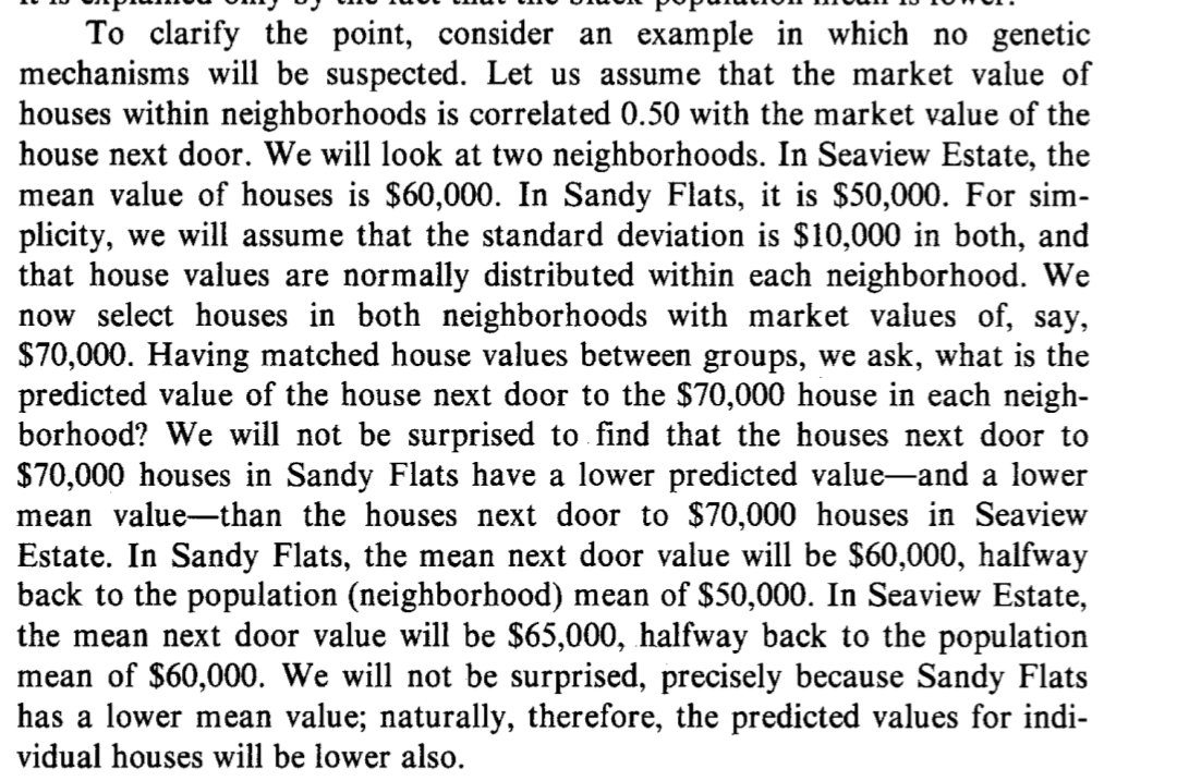
This is a general statistical property that does not require any particular causal explanation. Now, hereditarians argue that parents with high IQs will have children with somewhat lower IQs, and parents with low IQs will have children with somewhat higher IQs—both regressing toward the mean. They observe that the siblings of high-IQ black individuals regress further than the siblings of high-IQ white individuals—that is, if you find a black person and a white person both with IQs of 110, the black person’s sibling will tend to have a lower IQ than the white person’s sibling. The hereditarian takes this as evidence that the two groups have different genetic means.
There is much that could be said here, but the essential point is this: regression can only happen toward the population mean. The black sibling regresses toward the black mean; the white sibling regresses toward the white mean. We already know the two means are different—that is what everyone is trying to explain. This means that the regression-to-different-means phenomenon reduces to the black-white IQ gap itself: whatever causes the gap (whether genetic or environmental) will produce exactly this pattern of differential regression. If the gap is entirely environmental—if black Americans score lower because of environmental disadvantage—then high-scoring black individuals are further from their population mean than equivalently-scoring white individuals, and their siblings will regress more. The pattern provides no independent evidence for either a genetic or an environmental cause. It is circular: it assumes the very thing it purports to prove.
Whatever the cause of the gap, the regression-to-the-mean phenomenon is irrelevant to what adoption studies show. Regression to the mean is not about a process of IQ fadeout where gains are lost towards the population means but about a general statistical phenomenon that extreme outcomes are likely to be followed by more average outcomes. Adoption changes the environment, and the question is whether that environmental change shifts the group mean. Regression to the mean tells us nothing about whether environmental interventions work. It is a distraction in this context, and hereditarians who invoke it in response to adoption data are changing the subject.
3.11 Global IQ Scores - AI gen
[Add to this or to Jensen’s bias that online hereditarians sometimes treat IQ as meaning the same thing practically, e.g., IQ < 70 is mentally retarded, when showing IQ distributions online for black-white differences. In which case, the critique of countries being mentally retarded or of blacks making better use of their IQ points fully applies.]
Sometimes, hereditarians cite global IQ scores to provide evidence for their claim that the gap is primarily due to genetics. The argument is intuitive: if the same ranking of IQ scores for races occurs throughout the world, across many different countries and environments, what else could explain it but genetics? Much could be said about these global IQ scores, but we will have a brief treatment here. It is sufficient to show that the data cannot bear the weight the hereditarian places upon it.
The data itself cannot be trusted. The global IQ scores that hereditarians cite originate in the work of Richard Lynn, whose data collection methods were not merely imperfect but systematically flawed. Lynn and Vanhanen published national IQ estimates for 185 countries, but actual IQ data existed for only about 81 of them. The remaining 104 countries were “estimated” by averaging scores from neighboring nations—a procedure that assumes the conclusion the hereditarian wants to draw (that geography determines IQ) in order to fill in the data [Lynn, R., & Vanhanen, T. (2002). IQ and the Wealth of Nations. Praeger; Lynn, R., & Vanhanen, T. (2006). IQ and Global Inequality. Washington Summit Publishers]. Where data did exist, the samples were frequently absurd. The IQ estimate for Equatorial Guinea—at one point the lowest in the dataset—was derived from a sample of 48 children in a home for the developmentally disabled in Spain, who were not even from Equatorial Guinea [MacEachern, S. (2006). “Africanist archaeology and ancient IQ: Racial science and cultural evolution in the twenty-first century.” World Archaeology, 38(1), 72–92] [verify MacEachern exact citation; also cited in Wicherts et al. 2010]. The estimate for Ethiopia came from illiterate Beta Israel children who had just emigrated from rural Ethiopia to urban Israel—a sample selected for maximum cultural dislocation [Berhanu, G. (2007); Hunt, E., & Wittmann, W. (2008)] [verify exact citations]. For Nigeria, Lynn selected the lowest-scoring studies while ignoring published studies showing considerably higher averages [Wicherts et al. 2010]. For South Africa, one contributing sample consisted of just 17 illiterate children. Angola’s national IQ was based on 19 participants from a malaria study. Eritrea’s estimate came from children in orphanages [Sear, R. (2022). “‘National IQ’ datasets do not provide accurate, unbiased or comparable measures of cognitive ability worldwide.” Psychological Science — verify exact journal].
Wicherts, Dolan, and van der Maas (2010) conducted a systematic review of the IQ literature for sub-Saharan Africa and concluded that the average IQ was approximately 80—thirteen points higher than Lynn’s estimate of 67 [Wicherts, J. M., Dolan, C. V., & van der Maas, H. L. J. (2010). “A systematic literature review of the average IQ of sub-Saharan Africans.” Intelligence, 38(1), 1–20] [verify exact citation]. They found that Lynn’s methodology for selecting studies was not clearly specified: no inclusion or exclusion criteria were published, and no list of excluded studies with reasons for exclusion was provided. When Wicherts et al. used independent raters to evaluate the representativeness of the samples Lynn included and excluded, they found that the standard criteria for representativeness—whether the sample was randomly drawn, whether the original authors considered it representative, whether participants were healthy—had no bearing on whether Lynn included a study. The single best predictor of whether a study was included in Lynn’s dataset was whether it showed a low IQ score [Wicherts, J. M., Dolan, C. V., & van der Maas, H. L. J. (2010). “The dangers of unsystematic selection methods and the representativeness of 46 samples of African test-takers.” Intelligence, 38(1), 30–37]. That is not science. That is confirmation bias with a dataset.
The subsequent version of the dataset, maintained by David Becker, inherited these problems. Sear (2022) provided a thorough evaluation of the 2019 edition and found that it remained “not only inaccurate but systematically biased”—the dataset did not provide “comparable, accurate and unbiased measures of cognitive ability worldwide” [Sear 2022] [verify exact journal; may be a preprint or published in Intelligence or elsewhere]. As Sear noted, it is “wholly implausible that an entire world region should, on average, be on the verge of intellectual impairment”—which is precisely what Lynn’s estimates imply for sub-Saharan Africa. The hereditarian is aware of this implausibility. The standard response draws on Jensen’s distributional argument, which we discussed in our treatment of measurement invariance. Jensen argued that when a population has a lower mean, individuals at a given score are more likely to be there from ordinary variation rather than organic pathology, and therefore function better in daily life than individuals at the same score from a higher-mean population. Applied to sub-Saharan Africa, the argument runs: an average IQ of 70 does not imply that half the population is intellectually disabled, because most of those low scores reflect normal variation, not pathology. These individuals can function in their societies despite low scores on tests of abstract reasoning.
Grant this for the sake of argument. The distributional logic succeeds in dissolving the disability objection—but it creates a different problem. Hereditarians do not cite global IQ scores merely to report that certain populations score lower on abstract reasoning tests. That would be a thin, near-tautological claim. The substantive hereditarian thesis—stated explicitly in Lynn and Vanhanen’s IQ and the Wealth of Nations (2002) and running through the HBD literature—is that low IQ scores explain sub-Saharan African poverty, underdevelopment, and civilizational differences. The scores are cited as evidence not just of a test-score ranking but of a functional cognitive deficiency with real-world consequences.
Jensen’s distributional logic, applied at the level of means, undermines exactly this inference. If you have conceded that IQ 70 in a population with mean 70 does not predict the functional impairment that IQ 70 predicts in a population with mean 100—if you have conceded that these individuals can farm, trade, raise children, and maintain social institutions despite their scores—then you have conceded that the scores do not carry the practical weight you need them to carry. You can still say “they scored lower on this test.” You cannot then say “and that is why they are poor,” because you have just told us the scores do not predict practical outcomes the same way. And indeed, sub-Saharan African populations do maintain complex societies, agricultural systems, trade networks, and—as we document at length in our discussion of African history—they have built and administered empires, judicial systems, and diplomatic networks that are flatly inconsistent with population-wide cognitive deficiency of any kind. Either the scores reflect real functional deficiency (in which case these achievements are inexplicable) or they do not (in which case stop citing them as though they do). The hereditarian cannot have it both ways.
To be clear: this dilemma does not by itself refute the hereditarian claim that the ranking is global and therefore genetic—that claim we address below with the UK and immigrant data. What it does is strip the global IQ scores of the practical explanatory power the hereditarian wants them to have. Even if the ranking were universal (and we will see that it is not), the scores could not do the work the hereditarian assigns to them.
The hereditarian may respond that the scores are “still roughly right”—that quibbling over whether sub-Saharan Africa averages 67 or 80 does not change the basic picture of a global ranking. This response does not survive scrutiny. If the data collection method is systematically biased—selecting studies that confirm the researcher’s expectations and excluding those that do not—the results cannot be selectively trusted where they happen to confirm one’s priors. The burden is on those who wish to use the data to show it is reliable, and Wicherts and Sear have shown it is not. A dataset in which the best predictor of inclusion is whether the study supports the compiler’s thesis is not a dataset; it is an exercise in circular reasoning.
Moreover, even the corrected estimate of 80 must be understood in context. Sub-Saharan African nations have among the world’s lowest levels of education, nutrition, healthcare, and economic development. The Flynn Effect—sustained IQ gains averaging approximately 3 points per decade throughout the 20th century in industrialized nations—is far too rapid to reflect genetic change, and the leading explanations are environmental: improved nutrition, expanded education, reduced disease burden, removal of toxins, and the increasing cognitive complexity of daily life. As we documented above, Bratsberg and Rogeberg (2018) demonstrated through within-family analyses that both the Flynn Effect and its reversal are environmentally driven. Cumulative gains of 15 to 20 points have been documented in developed countries over the 20th century. As Flynn himself observed: scored against modern norms, Americans from a century ago would have averaged approximately IQ 70—the same figure Lynn assigns to sub-Saharan Africa [Flynn, J. R. (2007). What Is Intelligence? Beyond the Flynn Effect. Cambridge University Press] [verify: confirm this claim appears in the 2007 book; Flynn’s 2013 TED Talk states it explicitly, but the book is the better citation]. Herrnstein and Murray themselves acknowledged the absurdity of taking such scores at face value, writing that when one considers the science, literature, and arts of previous generations, one does not get the impression of diminished intellect [Herrnstein & Murray 1994, pp. 308–9; noted by MacEachern 2006, p. 84]. The hereditarian applies a standard to sub-Saharan African populations that he would not apply to his own great-grandparents.
The Flynn Effect has been documented within sub-Saharan Africa itself. Daley et al. (2003) measured cognitive gains among rural Kenyan children in Embu between 1984 and 1998 and found a gain of approximately 26 IQ points on Raven’s Progressive Matrices over just 14 years—a rate of nearly 2 points per year, far exceeding any gain ever recorded in the developed world (the composite gain across all tests was approximately 11 points; the Raven’s gain was larger because Raven’s is more sensitive to environmental change) [Daley, T. C., Whaley, S. E., Sigman, M. D., Espinosa, M. P., & Neumann, C. (2003). “IQ on the Rise: The Flynn Effect in Rural Kenyan Children.” Psychological Science, 14(3), 215–219]. The children’s average on Raven’s rose from approximately IQ 70 to approximately IQ 80 over that period. The causes Daley et al. identified—improved maternal education, better childhood nutrition and health, shifts in family structure—are environmental factors that remain dramatically worse in much of sub-Saharan Africa than in the developed world. A population currently scoring 80 under these conditions is not a population whose genetic potential is 80; it is a population whose environmental conditions have not yet caught up. The hereditarian treats a snapshot of current scores as a photograph of genetic capacity. The Flynn Effect—documented in Africa itself, at rates exceeding the developed world—shows it is a frame from a moving picture.
The ranking is not truly global. The hereditarian argument from global IQ data rests on the claim that the racial ranking—East Asians above whites above blacks—persists everywhere, regardless of environment, and that this consistency points to genetics. But the ranking does not persist everywhere. Counter-evidence from the United Kingdom is particularly damaging to this claim.
In England, all students take the General Certificate of Secondary Education (GCSE) examinations at approximately age 16. These are high-stakes, nationally administered exams covering core academic subjects. Unlike an IQ test administered to a small research sample, GCSEs are taken by virtually the entire student population—hundreds of thousands of students per ethnic group. By the end of secondary school in 2023, the majority of ethnic groups attained higher GCSE grades than White British pupils [Education Policy Institute, Annual Report 2024: Ethnicity]. By 2024, the Education Policy Institute reported that Black African students had overtaken White British students in GCSE attainment, as had Pakistani, Bangladeshi, and several other groups [Education Policy Institute, Annual Report 2025: Ethnicity]. On the GCSE English and maths combined pass rate (Grade 4 or above), Black African pupils achieved 69.4%—higher than the national average of 65.1% and higher than the White British rate of 63.6% [GOV.UK Ethnicity Facts and Figures, “GCSE English and Maths Results,” Key Stage 4 Performance, Academic Year 2022/23; UK Department for Education]. The White major ethnic group has the lowest pass rate on this combined measure among the five major ethnic groups tracked by the government (White 63.7%, Mixed 64.9%, Other 64.2%, Black 65.0%, Asian 74.8%), though this aggregate is pulled down by the Gypsy/Roma subgroup (16.2%); the White British subgroup specifically scores 63.6%, still below every non-White major group except Black Caribbean (52.1%) [same source]. In the 2019 data, the UK government’s own Commission on Race and Ethnic Disparities reported that “in terms of the percentage of students achieving a strong pass in Maths and English at GCSE, the White British group ranks 10th in attainment” [Commission on Race and Ethnic Disparities, “Education and Training,” 2021]. White British students are in the bottom half of the attainment distribution among ethnic groups in their own country.
Perhaps most striking is the performance of disadvantaged students. Black pupils eligible for free school meals (FSM)—a standard indicator of poverty in England—have a significantly higher GCSE pass rate in English and maths than the national average for all FSM-eligible pupils [House of Commons Library, “Educational outcomes of Black pupils and students,” CBP-9023, 2023]. This is not an artifact of immigrant self-selection into wealthy neighborhoods. These are the poorest Black students outperforming the average poor student of any ethnicity.
The hereditarian will object that the GCSE is not an IQ test. This is true in the narrow sense: GCSEs are achievement examinations, not psychometric instruments designed to measure g. But this objection is a double standard. We established in our earlier discussion that IQ tests are validated by their correlation with other cognitive measures, and that anything sufficiently correlated with an IQ test is treated as an IQ proxy by hereditarians themselves. The SAT is an achievement test; Murray uses AFQT scores (an achievement test) as the primary measure of cognitive ability in The Bell Curve; hereditarians routinely cite educational attainment as a proxy for IQ throughout the literature. The GCSE correlates strongly with formal cognitive tests: the CAT4 (Cognitive Abilities Test), a standardized cognitive assessment widely used in UK schools, correlates at r = 0.72 with GCSE Attainment 8 scores, with individual subject correlations reaching into the 0.60s and 0.70s (English Language 0.62, Computer Studies 0.65) [GL Assessment, “CAT4 UK Technical Report,” 2021, Table: Correlations of CAT4 and GCSE grades]. The CAT measures the same reasoning abilities assessed by standard IQ tests—verbal, non-verbal, quantitative, and spatial reasoning—and is described by GL Assessment as “the UK’s most widely used test of reasoning abilities” [GL Assessment, CAT4 product documentation]. [Flag: Gusev cites a CAT3-WISC correlation of r = 0.82 on X/Twitter, Feb 3, 2024; I have been unable to trace this to a primary source. The GL Assessment CAT4 UK Technical Report does not report a WISC correlation. If the primary source can be located, restore the specific figure here.] By the hereditarians’ own criteria, the GCSE is as much an IQ proxy as the SAT or AFQT. The hereditarian cannot accept the SAT as a cognitive measure when it shows a gap and reject the GCSE when it does not. That is not a methodological distinction. That is choosing whichever test confirms one’s priors.
A more sophisticated version of this objection points to the CAT (Cognitive Abilities Test), administered in some UK schools, which does show a Black-White gap more consistent with IQ test data. The hereditarian reads this as the CAT measuring “true” cognitive ability while the GCSE is inflated by effort and preparation. But the GCSE is a nationally administered exam taken by virtually all students, while the CAT is administered to a much more selected subset—it is primarily used to track cognitive ability in schools that choose to administer it, not a universal assessment. GL Assessment reports that over 750,000 students take the CAT4 each year [GL Assessment, CAT4 product page]—substantial, but well under the approximately 600,000 students per year group who sit the GCSE, and the selection of which schools administer the CAT is not random. The simplest explanation for the discrepancy is that the CAT is drawn from a more selected, less representative population, while the GCSE reflects the actual performance of the full national student body. A nationally administered test that matters for qualifications shows no gap; a more specialized test with a selected sample shows a gap; when the two are given to the same students, they are highly correlated—the CAT4 correlates at r = 0.72 with GCSE Attainment 8 scores [GL Assessment, “CAT4 UK Technical Report,” 2021]. The most parsimonious reading is that the CAT sample is unrepresentative, not that the GCSE is fraudulent. The hereditarian who insists otherwise needs to provide evidence that Black African students are systematically gaming the GCSE through superior “studiousness” rather than superior performance—and no such evidence has been provided [verify: has any peer-reviewed study demonstrated that Black African GCSE performance is inflated relative to cognitive ability? If such a study exists, it should be addressed]. The claim that the GCSE is “gameable” by studious minorities is asserted without evidence. And the pattern is predictable: whenever a test shows the expected gap, hereditarians treat it as a valid cognitive measure; whenever a test fails to show the gap, they reclassify it as an achievement test corrupted by effort. One can anticipate the same maneuver if SAT gaps narrow in the United States: the SAT will suddenly cease to be “mostly an IQ test” and become a mere achievement test gamed by preparation—despite hereditarians having treated it as a cognitive measure for decades [for the claim that the SAT is “mostly an IQ test,” see e.g. Cremieux on X/Twitter, May 17, 2023] [verify exact date and wording of tweet].
There is a subtler version of this objection worth addressing directly. The hereditarian might concede that the GCSE is cognitively demanding but argue that Black African immigrant families are selected for extreme academic motivation and discipline—a “tiger parent” cultural effect—and that this non-cognitive factor drives GCSE performance without requiring high cognitive ability. Two responses. First, if motivation and family academic culture can produce GCSE performance at or above the White British level despite a supposed genetic cognitive deficit of 15 to 30 IQ points, then those environmental and cultural factors are doing all the explanatory work. The genetic deficit, if it exists, is not producing the outcomes the hereditarian needs it to produce. This is not a defense of the hereditarian position; it is a concession of the environmentalist one. Second, the GCSE is not a test that rewards pure effort while bypassing cognition. GCSE Mathematics requires algebraic reasoning, geometric proof, and statistical inference; GCSE English requires textual analysis and argumentative writing; the sciences require experimental reasoning and quantitative problem-solving. These are cognitively demanding tasks, and the r = 0.72 correlation between the CAT4 and GCSE Attainment 8 confirms that what the GCSE measures overlaps substantially with what cognitive tests measure. A student cannot pass GCSE Mathematics through sheer diligence if she cannot reason algebraically. The “motivation not cognition” objection requires that an entire population is systematically outperforming another on cognitively loaded examinations through effort alone—a claim that, if true, would itself require explanation and would still not rescue the hereditarian’s genetic hypothesis.
To be fair: the overall picture in the UK is not uniformly favorable to Black students. Black Caribbean pupils still score below White British pupils on the GCSE, and at age 5, Black African children score below White British children—they catch up and overtake during the school years [Education Policy Institute, Annual Reports 2023–2025]. The pattern is complex, and the variation among Black subgroups is itself informative: if the gap were primarily genetic, one would not expect Black African students (who are predominantly children of recent immigrants from sub-Saharan Africa and thus carry little or no European admixture [verify: demographic composition of UK “Black African” category; this is the standard understanding but cite ONS or Census data]) to outperform White British students while Black Caribbean students (who carry significant European admixture from the colonial period, typically estimated at 10–20% [verify: admixture estimates for Caribbean-descended populations in UK]) do not. The hereditarian predicts that more African ancestry means worse cognitive outcomes. The UK data shows the opposite: the group with more African ancestry outperforms the group with less. The hereditarian prediction runs exactly backward.
Second-generation African immigrants in the United States present a similar problem for the hereditarian. African immigrants and their children in the United States show educational achievement that matches or exceeds the White American average. Nigerian Americans in particular are among the most educated ethnic groups in the country [verify: U.S. Census data on Nigerian American educational attainment; widely cited but verify specific source]. Even using the hereditarian’s own proxy methods—identifying Nigerian Americans among National Merit Scholarship semifinalists by surname—the estimated cognitive ability of Nigerian Americans is approximately at parity with the White American average, with the gap between the two groups falling within the range of statistical noise (approximately 0.03 standard deviations, or less than half an IQ point) [Cremieux, “The Myth of Nigerian Excellence,” 2024; note that this is a hereditarian source, and the author’s own data shows essential parity, not a deficit] [verify: confirm whether the comparison baseline is the white mean or the population mean; the source states “contrasted with Whites”] This finding sits uncomfortably with the hereditarian claim that populations of sub-Saharan African ancestry carry a genetic cognitive deficit of 15 to 30 IQ points.
The hereditarian will raise the selection objection: immigrants are not representative of their home populations. This is true. Immigrants are selected for motivation, education, and often ability. But this objection does not rescue the hereditarian position for several reasons. First, the selection objection applies to the first generation—the adults who chose to immigrate. Their children, the second generation, did not select themselves. They were born and raised in the destination country and attended its schools. If a genetic cognitive deficit of the magnitude hereditarians claim were real, selection on parental motivation and education could not overcome it in a single generation. A population with a genetic IQ of 70 (Lynn’s estimate for Nigeria) cannot easily produce children who score at the White American average through selection effects alone—the arithmetic requires assumptions so extreme as to be self-defeating.[^selection_arithmetic] Second, even if we grant that immigrant parents are selected, the selection is primarily on education and motivation, not on IQ directly. This matters because education and motivation are environmental variables. If selection on these environmental traits is sufficient to produce a community whose children perform at the White average, the hereditarian has inadvertently demonstrated that environmental factors can close the gap — which is the environmentalist thesis. The hereditarian cannot simultaneously argue that the gap is genetically immutable and that non-genetic selection factors fully account for immigrant success. Third, and most directly: the UK data on free-school-meals-eligible Black students outperforming FSM-eligible White British students cannot be explained by immigrant selection into high socioeconomic status. These are the poorest students in the comparison. Whatever is driving their performance, it is not wealth.
The selection objection faces an additional problem specific to the UK data: the “Black African” category is not a single immigrant stream from a single country. It encompasses children whose families originate in Nigeria, Ghana, Sierra Leone, Zimbabwe, the Democratic Republic of Congo, Angola, Somalia, Ethiopia, Eritrea, Sudan, Kenya, Tanzania, and elsewhere [Demie & McLean, 2007; Demie, 2021, “The Educational Achievement of Black African Children in England”]. In a single London borough (Lambeth), GCSE-sitting Black African pupils speak over twenty different home languages, including Yoruba, Somali, Twi-Fante, Igbo, Krio, Tigrinya, Lingala, Ga, Swahili, Luganda, and Amharic [Demie 2021]. The migration pathways that produced this population are radically diverse: Nigerians often come as students or professionals; Somalis, Eritreans, and Congolese are frequently refugees who were selected for proximity to conflict, not for cognitive ability [Mitton & Aspinall, University of Kent; verify exact citation]. Cognitive selection cannot plausibly operate uniformly across all these populations, arriving through different pathways, from different countries, for different reasons, and yet the aggregate category outperforms White British students. Moreover, within the Black African category, the variation in attainment tracks environmental factors—principally English language proficiency—rather than country of origin in the pattern a genetic model would predict [Demie 2021]. Nigerian- and Ghanaian-origin children tend to outperform; Somali-origin children tend to underperform; but when English proficiency is accounted for, these gaps narrow substantially [Demie, “The Achievement of Somali Pupils in Lambeth Schools,” 2024] [verify exact citation]. The within-group variation is what an environmental model predicts and what a hereditarian genetic model does not. The regression-to-mean argument we develop below for Nigerian Americans applies with equal force here: UK Black African children are predominantly second-generation, and under the hereditarian’s genetic model, they should be regressing toward the sub-Saharan African genetic mean of 70—not outperforming the host population.
[^selection_arithmetic] Here is the problem. If the Nigerian population has a genetic mean IQ of 70 with a standard deviation of 15, then only about 2.3% of the population scores above 100. Suppose immigrant parents are drawn entirely from this cognitive elite—an extreme assumption, since Nigerian immigrants include students, workers, family-reunion migrants, and others who are not uniformly high-IQ. Grant it anyway. These selected parents average, say, IQ 105–110. Under the hereditarian’s own genetic model, their children should regress toward the population’s genetic mean. With a heritability of 0.5, children of parents averaging IQ 110 from a population with genetic mean 70 would be expected to average about 90—not 100. With a heritability of 0.8 (the upper end of twin-study estimates that hereditarians prefer), the expected second-generation mean would be about 102—but only if the parents averaged 110 and the trait is 80% heritable and every single immigrant was drawn from the top 2% of the Nigerian distribution. This is not a realistic scenario; it is the most favorable case imaginable, and it barely reaches parity. If the parents are even slightly less selected—as they certainly are in any real immigrant population—the second-generation prediction falls well below the white mean. The hereditarian can make the arithmetic work only by granting Nigerian immigrants a degree of cognitive selection so extreme that it implies a large, high-performing cognitive elite in Nigeria—which itself undermines the claim that the population is genetically constrained to low cognitive ability.
Non-immigrant evidence. The selection objection does not apply to all the relevant data. The Eyferth study (1961), discussed at length in our section on adoption, tested children fathered by American occupation soldiers and raised by white German mothers after World War II. Children of black American soldiers scored at essentially the same IQ (96–97) as children of white American soldiers raised in identical circumstances. These children were not immigrants. Their fathers were ordinary soldiers, not a selected cognitive elite. The hereditarian prediction—that the black-fathered children should score 7–8 points lower, reflecting the genetic contribution of their fathers—was excluded at conventional significance levels [see adoption section for full discussion, including the screening objection and its limitations]. Kirkegaard, Lasker, and Kura (2019) replicated the null result with biracial children of U.S. servicemen in post-war Japan—a concession from a hereditarian researcher. These results show that even outside the immigrant context entirely, the racial ranking is not fixed when rearing environments are equalized.
What follows from all this? We should be clear about what we have and have not shown. We have not shown that there is no IQ gap in any country, or that global IQ scores are meaningless noise. There are real differences in cognitive test performance across countries and populations, and those differences correlate with real differences in development, education, nutrition, and economic opportunity. What we have shown is that the hereditarian’s favored dataset is unreliable, that its compiler selected data in a manner that systematically depressed African scores, that the “global ranking” does not hold in the one country where we have the best data on Black and White academic performance in a shared educational system, and that populations of African descent regularly match or exceed White performance when environmental conditions permit. The global IQ data does not support the hereditarian thesis. It is not evidence for a genetic racial hierarchy. It is evidence that environmental conditions vary across the world—which no one disputes.
3.12 What Genetics Predicts: The Neutral Bound Applied to IQ - AI gen
We have investigated the evidence from social science about the causes of the IQ gap. We have found that IQ is malleable, that gains can be persistent, that environmental factors explain large portions of or most of the gap, that education has a causal relationship with IQ, and that the direct evidence from adoption studies—though ultimately inconclusive—contradicts specific hereditarian claims and provides evidence of the environmentalist thesis. We come at last to the calculation of what genetics can contribute to the IQ gap using the neutral theory we explained in our earlier section on genetics [add link to section]. We will find that the expected genetic contribution from drift is small—a few IQ points at most—and could favor either group. The single most probable genetic contribution is zero. The hereditarian thesis that 50% or more of the gap is genetic requires an improbable tail of the drift distribution.
3.12.1 The Parameters
We need two inputs: the direct heritability of IQ and FST between U.S. blacks and whites.
Direct heritability. Direct effects are what we want, because this is the state of the question between hereditarians and environmentalists: how much of the IQ gap is caused by genetics? How much of the gap is immutable because caused by genetics? Direct heritability is estimated from within-family methods—comparing siblings who share the same family environment but received different random draws of parental alleles—and the estimates are considerably lower than the twin-study values hereditarians typically cite.
Two large-scale within-family GWAS analyses have estimated the direct heritability of cognitive performance, both using LD-score regression (LDSC) to convert effect sizes into heritability estimates. Howe et al. (2022, Nature Genetics) reported a direct h² of 0.14 (population h² of 0.24, an attenuation of 42%) [cite]. Tan et al. (2024, medRxiv) reported a direct h² of approximately 0.19 [cite]. However, LDSC is known to inflate heritability estimates: Hou et al. (2019) benchmarked it against simulated ground truth and found a systematic overestimate of 1.47–1.86× on average. A more accurate variant, stratified LDSC (S-LDSC), eliminated most of this bias (ratio of 1.001 on average).
Gusev (2024) reanalyzed both data sets using S-LDSC https://theinfinitesimal.substack.com/p/what-are-we-learning-from-the-genes. The results converged downward. For Howe et al., Gusev’s LDSC reproduction yielded 0.13 for the direct estimate (close to the published 0.14), but S-LDSC reduced it to 0.11. For Tan et al., Gusev’s LDSC reproduction yielded 0.17 for the direct estimate—lower than the published 0.19, suggesting a possible methodological discrepancy in the original analysis—and S-LDSC reduced it further to 0.12 [cite Gusev blog]. In both cases, S-LDSC produced estimates with wide confidence intervals, but the central values converged: the direct heritability of cognitive performance is approximately 0.11–0.12 by the most accurate available method.76
These results mean the best current estimate for the direct heritability of IQ is h² ≈ 0.11–0.12 (using S-LDSC), with standard LDSC giving values up to 0.17. A reasonable range is thus h² = 0.11–0.17. Readers who find these values surprisingly low compared to the 0.50–0.80 range from twin studies should review our earlier discussion of heritability, where we showed why twin-study estimates are systematically inflated by confounders that molecular methods remove [add link to heritability section]. In what follows, we will use h² = 0.15 as a central estimate and h² = 0.20 as a generous upper bound—above all current estimates but allowing for residual uncertainty. We will also compute results for h² = 0.25, 0.30, and 0.50 (the latter being the lower limit of twin-study estimates that hereditarians cite) for comparison.
A hereditarian might object that the “real” heritability is much higher because current molecular methods miss rare genetic variants. This objection has been directly tested. Bird (2026) used population-genetic theory—calibrated against empirically measured distributions of selection coefficients [Simons et al. 2025; Zhu et al. 2026]—to estimate how much heritability sits in variants too rare for current genotyping arrays to detect. The answer: roughly 9–25% of total heritability, depending on the selection model. For brain-related traits specifically, it is approximately 9%. These predictions are confirmed by whole-genome sequencing data [Wainschtein et al. 2026; Wang et al. 2026]. Rare variants simply cannot close the enormous gap between twin-study estimates (50–80%) and molecular estimates (11–17%). The most parsimonious explanation is that twin studies systematically overestimate heritability because they assume genes and environment do not interact or correlate—assumptions that are known to be violated for cognitive and socioeconomic traits [see our earlier discussion of heritability, add link; Bird 2026 https://sequencesandconsequences.substack.com/p/is-missing-heritability-actually].
There is therefore no reason to believe h² will reach beyond 0.20 for IQ, and values of 0.25 or higher should be understood as extreme scenarios included for completeness.
FST. Next, we need the genome-wide FST between U.S. blacks and whites. The relevant measure is the Hudson FST, a pairwise estimator recommended by Bhatia et al. (2013, Genome Research) and used by Gusev in the framework we are applying [see Technical Notes below]. The 1000 Genomes Phase 3 data give a genome-wide Weir-Cockerham FST of 0.090 between African Americans (ASW) and Northern European Americans (CEU), which is approximately equal to the Hudson FST for balanced samples [Auton et al. 2015; Bhatia et al. 2013]. This value is consistent with what we would expect from the underlying continental divergence: the CEU–YRI (European–Yoruba) FST from 1000 Genomes is approximately 0.14, and U.S. African Americans carry substantial European ancestry—estimates range from roughly 17% to 24% depending on the sample and method [Bryc et al. 2010; Bryc et al. 2015; Baharian et al. 2016]—which reduces the effective pairwise FST [see Technical Note C]. In what follows, we present results for FST = 0.08 and 0.10. The empirical estimate of 0.090 falls between these values. FST = 0.10 is conservative—approximately 11% above the empirical estimate—and makes the neutral bound more generous to the hereditarian position. FST = 0.08 represents the lower bound of the plausible range, corresponding to the higher admixture estimates; results at this value are included to show the full range of plausible values.
3.12.2 The Equations
Under the neutral model, the proportion of total phenotypic variance in IQ attributable to genetic differences between the two populations is:
\[ R = \frac{F_{ST} \cdot h^2}{1 - F_{ST} + F_{ST} \cdot h^2} \tag{1}\]
This is derived from the Edge & Rosenberg (2015a, 2015b) framework for neutral polygenic traits, extended to traits with h² < 1 [see Technical Notes below]. For small values of FST × h², this simplifies to R ≈ FST × h², the approximation used by Gusev. At our parameter values, the denominator correction adds roughly 5%, which is small but worth including for exactness.
The genetic gap between the two populations—the difference in group means attributable to neutral genetic drift—is a random variable centered at zero. Its standard deviation (RMS) is:
\[ \Delta_{RMS} = 2\sigma\sqrt{R} \tag{2}\]
where σ = 15 is the conventional IQ standard deviation [see Technical Notes on this choice]. And the expected absolute magnitude—the average size of the genetic gap across many independent neutral traits, ignoring direction—is:
\[ E[|\Delta|] = \sqrt{\frac{2}{\pi}} \cdot \Delta_{RMS} \approx 0.798 \cdot \Delta_{RMS} \tag{3}\]
3.12.3 What These Quantities Mean
Imagine surveying many traits in two populations whose allele frequencies have drifted apart. For each trait, we compute the genetic difference between the populations: positive when population A is favored, negative when population B is favored. Sometimes the difference is large, sometimes small, sometimes near zero. When we average these signed differences across many traits, we get zero—drift favors neither population systematically. The expected signed difference is 0.
But the differences are not all zero individually. How big are they typically? Two measures tell us.
The expected absolute difference (E[|Δ|]) is the simple average of the magnitudes—ignoring whether population A or B is favored. If we surveyed 100 neutral traits, added up the absolute size of each genetic gap, and divided by 100, we would get approximately E[|Δ|]. This is the intuitive “average drift effect.” At central parameter values, it is about 3 IQ points.
The RMS (ΔRMS) is a different kind of average. It squares each deviation, averages the squares, and takes the square root—a “quadratic average” that gives extra weight to occasional larger deviations. When the mean is zero, as it is here, the RMS equals the standard deviation. It is roughly 25% larger than the simple average because of the extra weight given to the tails. In electrical engineering, the RMS is used to express the “effective magnitude” of an alternating current—the DC equivalent that delivers the same power. In our context, the RMS is the “effective scale” of drift: it captures the full spread of possible outcomes, including the occasional larger ones. Because it equals the standard deviation, it directly gives us probability intervals: 68% of neutral outcomes fall within ±ΔRMS of zero, and 95% fall within ±1.96 × ΔRMS.
The most probable genetic difference for any single trait is zero. The expected absolute difference tells us what we typically observe. The RMS tells us the spread of possibilities. Neither is “the” answer; together, they describe the full distribution of what drift can do.
3.12.4 Results
[Table 1 should be inserted here]
| FST | h² | R | E[|Δ|] (d) | ΔRMS | 95% bound | P(Δ > 7.5) | P(Δ > 9) |
|---|---|---|---|---|---|---|---|
| 0.08 | 0.12 | 1.0% | 2.4 (0.16) | 3.1 | ±6.0 | 0.7% | 0.2% |
| 0.08 | 0.15 | 1.3% | 2.7 (0.18) | 3.4 | ±6.7 | 1.4% | 0.4% |
| 0.08 | 0.20 | 1.7% | 3.1 (0.21) | 3.9 | ±7.7 | 2.8% | 1.1% |
| 0.10 | 0.12 | 1.3% | 2.7 (0.18) | 3.4 | ±6.7 | 1.5% | 0.4% |
| 0.10 | 0.15 | 1.6% | 3.1 (0.20) | 3.8 | ±7.5 | 2.5% | 1.0% |
| 0.10 | 0.20 | 2.2% | 3.5 (0.24) | 4.4 | ±8.7 | 4.5% | 2.1% |
| 0.10 | 0.25 | 2.7% | 3.9 (0.26) | 4.9 | ±9.7 | 6.4% | 3.4% |
| 0.10 | 0.30 | 3.2% | 4.3 (0.29) | 5.4 | ±10.6 | 8.2% | 5.8% |
| 0.10 | 0.50 | 5.3% | 5.5 (0.37) | 6.9 | ±13.5 | 13.8% | 9.5% |
Table 1. Neutral genetic bound on the IQ gap for U.S. Black and White populations. Bolded rows show the most defensible parameter ranges (h² = 0.15–0.20, FST = 0.08–0.10). Italicized rows are included for comparison at higher h² values not supported by current evidence. R = proportion of phenotypic variance explained by genetic variation as a percent. E[|Δ|] = expected absolute genetic gap in IQ points, with Cohen’s d in parentheses. ΔRMS = standard deviation (RMS) of the genetic gap. 95% bound = ±1.96 × ΔRMS. P(Δ > 7.5) and P(Δ > 9) = one-tailed probability that drift produces a genetic gap of at least 7.5 or 9 IQ points in a specific direction (corresponding to 50% of the standard 15-point hereditarian gap and 50% of the wider 18-point white-specific gap, respectively).
3.12.5 Interpretation
What do these results tell us?
The expected genetic contribution from drift is small. At the central parameter values, i.e., the conservative FST of 0.10 and the best-supported heritability range (h² = 0.15–0.20), the expected absolute genetic gap is about 3–3.5 IQ points, representing 20–23% of the standard 15-point gap. This is a small effect by Cohen’s conventions (d = 0.20–0.24), and it could favor either population with equal probability. To put this in perspective, Charles Murray himself has conceded that a group difference of d = 0.3 “wouldn’t be worth worrying about except for the size of the tails” [Murray, X post, May 16, 2026 https://x.com/charlesmurray/status/2055677794286272543; see our earlier discussion of what constitutes a meaningful group difference, add link]. The neutral bound predicts a genetic difference well within Murray’s own threshold for irrelevance.
The most probable genetic contribution is zero. Under neutrality, the genetic gap is drawn from a normal distribution centered at zero. Zero is the single most probable value. The expected absolute difference of ~3 points is an average across many possible neutral traits or drift histories; for IQ specifically, the actual genetic contribution could be zero, could be 2 points favoring whites, could be 4 points favoring blacks. The neutral model does not predict any particular outcome—it predicts a distribution of possibilities, and the center of that distribution is zero.
The proportion of variance explained is negligible. The genetics associated with one’s ancestral background—what we loosely call race—account for 1–2% of the total differences in IQ among all individuals in both populations. The remaining 98–99% is due to other factors: individual genetic variation, environment, measurement error. As we have seen repeatedly throughout this paper, there is far more variation within groups than between them.
The hereditarian thesis requires an improbable tail scenario. The hereditarian thesis, as formulated by Jensen (1969) and Murray/Herrnstein (1994), holds that roughly 50% of the Black–White IQ gap is attributable to genetic differences.77 At central parameter values (FST = 0.10, h² = 0.15), this claim requires a genetic gap of 7.5 IQ points in a specific direction—favoring whites, not blacks. Under the neutral model, the probability of drift producing a gap this large in a specific direction is approximately 2.5%. At our generous upper-bound h² of 0.20, the probability rises to 4.5%—still well under 5%. Using the wider white-specific gap of 18 points, the hereditarian claim of 50% genetic requires 9 IQ points, with a probability of just 1.0–2.1%.
These are one-tailed probabilities. Under neutrality, the genetic gap is drawn from a normal distribution centered at zero. Any drift outcome is equally likely to favor Black or White populations. When we ask “what is the probability that drift produces a gap of at least 7.5 IQ points favoring whites specifically?”, we are looking at one tail of the distribution. The probability of a 7.5-point gap in either direction is double the values reported in the table (roughly 5–9% at central parameters). But the hereditarian thesis is directional—it claims whites are genetically advantaged in IQ, not merely that some gap exists. The one-tailed probability is the relevant test.78
We can also think of our results in terms of hypothesis testing. Take the neutral model as the null hypothesis and ask: is the hereditarian claim consistent with the range of outcomes neutrality predicts?
The 95% prediction interval in the table is two-tailed: it shows the range within which 95% of neutral drift outcomes fall, with 2.5% of outcomes in each tail. This interval is useful for understanding the general spread of drift, but it is not the right test for the hereditarian thesis. The hereditarian claim is directional—it does not merely assert that some large genetic gap exists in some direction, but that whites are specifically genetically advantaged in IQ. To test a directional claim, we use a one-tailed test, which concentrates the full 5% rejection threshold in the relevant tail. The one-tailed 95% boundary (1.645 × ΔRMS) is tighter than the two-tailed boundary (1.96 × ΔRMS), because all of the rejection power is focused in one direction rather than split across two.79
At our central parameters (FST = 0.10, h² = 0.15), the one-tailed 95% boundary is 1.645 × 3.84 = 6.3 IQ points. The 7.5-point hereditarian claim exceeds this boundary: it is rejected at α = 0.05 (one-tailed P = 0.025). At our generous upper-bound h² of 0.20, the boundary rises to 1.645 × 4.42 = 7.3 points—the 7.5-point claim just barely exceeds it (one-tailed P = 0.045). At our lower FST estimate of 0.08 with h² = 0.15, the boundary is just 5.6 points and rejection is comfortable (P = 0.014). The 9-point hereditarian claim (50% of the wider 18-point white-specific gap) is rejected at α = 0.05 for every defensible parameter combination; it enters the one-tailed 95% interval only at h² ≥ 0.25, above all current molecular estimates.
To summarize: under the two-tailed 95% interval, the 7.5-point hereditarian thesis barely fits inside the predicted range at some parameter values—meaning that a gap of this magnitude in some direction is not quite extraordinary enough to rule out. But under the one-tailed test appropriate to the directional hereditarian claim, the thesis is rejected at the conventional 5% significance level across all central parameter values. The hereditarian thesis sits right on the knife’s edge of what the neutral model permits, and falls outside when tested with the directional precision the claim itself demands.
It is worth pausing on what this probability means. Unlike the individual-level probabilities we computed in the ministerial fitness section, where the large Black population ensures that even low-probability outcomes are realized by many individuals, the drift scenario for IQ is a single draw. IQ is one trait; the drift history that produced whatever genetic difference exists between these populations happened once. A 2.5% probability is genuinely a 1-in-40 scenario, not a per-person probability that gets multiplied across millions of people. The hereditarian needs this one specific trait to have landed in the tail of its distribution, in the right direction.80
At higher heritability values that are not supported by current evidence but that we include for completeness, the hereditarian thesis becomes less improbable: at h² = 0.25, the probability rises to 6.4% for the 7.5-point target. Even here, the hereditarian thesis sits in the outer tail. And h² = 0.25 is itself above all current molecular estimates of the direct heritability of IQ. Only at h² = 0.50—the twin-study value that requires ignoring all the evidence for confounding in twin designs—does the hereditarian thesis become comfortable. When the upper bound of the neutral model just barely includes the lower bound of the hereditarian theory, and only at parameter values that are themselves above the best current estimates, this is a mark against the theory, not for it [cf. Bird 2021].
This calculation is an upper bound. The neutral bound assumes no gene-environment interaction (GxE). If GxE is present—as evidence suggests it is for cognitive traits [Turkheimer et al. 2003; Mostafavi et al. 2020]—then the portable, environment-independent genetic contribution to group differences is smaller than what we computed. GxE means that genetic effects depend on environment: the same allele-frequency differences can produce a smaller, larger, or even reversed phenotypic difference in different environments. If we change the environment, the genetic effects change too. This is not the immutable genetic ceiling that the hereditarian thesis requires. Because our calculation assumes all genetic effects are additive and environment-independent, the computed values should be understood as an upper bound on the direct genetic contribution to the gap, not a point estimate. The true genetic contribution is likely smaller.
Furthermore, as discussed above, the h² values we use likely retain some residual upward bias even after S-LDSC correction. The Mexico City admixture study [Wang, Visscher, et al. 2025, medRxiv], which used within-family methods to separate genetic from environmental effects of ancestry on educational attainment, found that the ancestry-education association vanished entirely within families—even though the ancestry-height association survived, as the neutral model predicts for a trait with genuine genetic differentiation [see our earlier discussion of admixture studies, add link]. The empirical evidence and the theoretical calculation converge: the expected direct genetic contribution to the cognitive gap between U.S. Black and White populations is small, most probably zero, and the hereditarian thesis of a large genetic component is improbable.
What can we conclude? The neutral model does not permit a deductive proof that the hereditarian thesis is false. We are dealing with probabilities, not certainties, and we say so plainly.81 What the evidence shows is this: at the best current estimates of direct heritability and population differentiation, the neutral model predicts that the genetic contribution to the IQ gap is most probably zero, typically around 3 IQ points in magnitude, could favor either population, and is small by any standard convention—well within the range that Murray himself concedes “wouldn’t be worth worrying about” [see our earlier discussion of group differences, add link].
The hereditarian thesis that 50% or more of the gap is genetic requires that drift produced a gap in the outer 2–5% of its probability distribution, in a specific direction, under the most defensible parameter values. At less defensible but higher h² values, the thesis becomes less improbable—but those parameter values are themselves implausible. When the upper bound of the neutral model just barely includes the hereditarian hypothesis, and only at h² values that exceed all current molecular estimates, this is not a close call. The thesis requires stacking assumptions: an h² at or above the top of the current range, a drift outcome in the tail, and a direction that happens to align with the observed gap. Each assumption individually is uncertain; their conjunction is improbable.
Moreover, every concession we have made in this calculation favors the hereditarian position. We used σ = 15 rather than the smaller within-group SD (~13.8), which inflates our bound by ~8%. We ignored gene-environment interaction, which would shrink the portable genetic contribution [see our earlier discussion of GxE, add link]. We used FST = 0.10, which is at the high end of empirical estimates. And we used h² values that likely still contain residual upward bias even after S-LDSC correction. If we must assume unreasonably high heritability and ignore gene-environment interaction to have the upper bound barely include the hereditarian hypothesis, the calculation is best understood as evidence against the thesis, not a close contest. The weight of the genetic evidence is against the hereditarian position. What remains—and what must do all the work—is the environmental explanation, which as we have seen throughout this paper is well-supported by direct evidence.
3.12.6 Technical Notes - AI gen
These notes provide mathematical detail for readers with some technical background. They may be skipped without loss of the main argument.
A. Derivation from Edge & Rosenberg. Edge & Rosenberg (2015a, 2015b) model a fully heritable, selectively neutral, additively determined polygenic trait in two populations. Their framework begins with a quantitative trait T determined entirely by genetics (T = G, i.e., h² = 1). Define:
- WG = within-population genetic variance (the average genetic variance within each population)
- BG = between-population genetic variance (the variance of population means) The proportion of total genetic variance that falls between populations is:
\[ \rho^2_T = \frac{B_G}{W_G + B_G} \tag{4}\]
Edge & Rosenberg prove that under selective neutrality, the expected value of ρ²T for diploids is approximately:
\[ E[\rho^2_T] \approx F^{(2)}_{ST,k} \tag{5}\]
where F(2)ST,k is the Hudson/diploid FST computed from the allele frequencies of the underlying loci. This is the key result: for a neutral trait, the fraction of genetic variance between groups tracks FST.
Now extend to a trait with h² < 1. Write the phenotype as P = G + E, where E is the environmental component. Within each population, the phenotypic variance is:
\[ W_P = W_G + W_E \tag{6}\]
and the within-population heritability is:
\[ h^2 = \frac{W_G}{W_P} \tag{7}\]
The between-population genetic variance BG is the same as in the fully heritable case—the environment does not create genetic differences between populations. From the definition of ρ²T:
\[ \rho^2_T = \frac{B_G}{W_G + B_G} \tag{8}\]
Solving for BG:
\[ B_G = \frac{\rho^2_T}{1 - \rho^2_T} \cdot W_G = \frac{F_{ST}}{1 - F_{ST}} \cdot h^2 \cdot W_P \tag{9}\]
where we substituted E[ρ²T] ≈ FST and WG = h² × WP.
We want R, the proportion of total phenotypic variance (not just genetic variance) attributable to between-group genetic differences:
\[ R = \frac{B_G}{W_P + B_G} \tag{10}\]
Substituting the expression for BG:
\[ R = \frac{\frac{F_{ST} \cdot h^2}{1 - F_{ST}} \cdot W_P}{W_P + \frac{F_{ST} \cdot h^2}{1 - F_{ST}} \cdot W_P} \tag{11}\]
Dividing numerator and denominator by WP:
\[ R = \frac{\frac{F_{ST} \cdot h^2}{1 - F_{ST}}}{1 + \frac{F_{ST} \cdot h^2}{1 - F_{ST}}} = \frac{F_{ST} \cdot h^2}{(1 - F_{ST}) + F_{ST} \cdot h^2} = \frac{F_{ST} \cdot h^2}{1 - F_{ST} + F_{ST} \cdot h^2} \tag{12}\]
For small FST × h², the denominator approaches 1, giving the first-order approximation R ≈ FST × h².
Finally, for two populations of equal size with a mean contrast Δ = μ₁ − μ₂, the between-group variance is B = Δ²/4. The total variance is σ²total = WP + BG. So:
\[ R = \frac{B_G}{W_P + B_G} = \frac{\Delta^2/4}{W_P + B_G} \approx \frac{\Delta^2}{4 \sigma^2} \tag{13}\]
where σ = 15 is the IQ standard deviation (using σ²total ≈ WP + BG ≈ WP since BG is small). Solving for the RMS of Δ:
\[ \Delta_{RMS} = 2\sigma\sqrt{R} \tag{14}\]
The expected absolute value of a zero-mean normal random variable with standard deviation σ_D is E[|D|] = √(2/π) × σ_D. Since Δ_RMS is the standard deviation of the genetic gap:
\[ E[|\Delta|] = \sqrt{\frac{2}{\pi}} \cdot \Delta_{RMS} \approx 0.798 \cdot \Delta_{RMS} \tag{15}\]
B. Relationship between Bird’s and Gusev’s formulas. Bird (2021) uses a QST-style parameterization. Define:
- σ²A = within-population additive genetic variance = h² × σ²P = WG
- σ²B = between-population genetic variance = BG Bird’s analog of FST for a quantitative trait is:
\[ Q_{ST} = \frac{\sigma^2_B}{2\sigma^2_A + \sigma^2_B} = \frac{B_G}{2W_G + B_G} \tag{16}\]
This is the QST formula for diploid organisms. The factor of 2 in the denominator arises because diploid individuals carry two copies of each allele, so the within-population genetic variance per allele copy is WG/2, and the total per-copy variance is WG/2 + BG/2. The ratio of between to total per-copy variance gives QST = (BG/2) / (WG/2 + BG/2) = BG / (WG + BG)… but wait, that gives the same denominator as ρ²T. The distinction is subtle: QST as traditionally defined [Spitze 1993; Whitlock 2008] uses the single-copy (haploid) variance partition:
\[ Q_{ST} = \frac{V_B}{V_B + 2V_W} \tag{17}\]
where VW is the additive genetic variance within populations. This maps onto Edge’s single-copy FST,k:
\[ F_{ST,k} = \frac{B_G}{2W_G + B_G} \tag{18}\]
while the diploid version used by Gusev is:
\[ F^{(2)}_{ST,k} = \frac{B_G}{W_G + B_G} \tag{19}\]
The two are related by:
\[ F^{(2)}_{ST,k} = \frac{2 F_{ST,k}}{1 + F_{ST,k}} \qquad \text{or equivalently} \qquad F_{ST,k} = \frac{F^{(2)}_{ST,k}}{2 - F^{(2)}_{ST,k}} \tag{20}\]
Bird sets QST equal to the FST computed from his SNP data and solves for σ²B:
\[ \sigma^2_B = \frac{2 F \cdot h^2 \cdot \sigma^2_P}{1 - F} \tag{21}\]
where F should be the Nei/single-copy FST,k. He then computes:
\[ \Delta_{RMS} = 2\sqrt{\sigma^2_B} = 2\sigma_P \sqrt{\frac{2F \cdot h^2}{1-F}} \tag{22}\]
Now substitute F = FST,k = FH / (2 − FH) to express Bird’s formula in terms of Hudson FST:
\[ \frac{2F_{ST,k}}{1 - F_{ST,k}} = \frac{2 \cdot \frac{F_H}{2-F_H}}{1 - \frac{F_H}{2-F_H}} = \frac{2F_H}{(2 - F_H) - F_H} = \frac{2F_H}{2(1-F_H)} = \frac{F_H}{1 - F_H} \tag{23}\]
So Bird’s formula becomes:
\[ \Delta^2_{RMS} = 4\sigma^2_P \cdot \frac{F_H \cdot h^2}{1 - F_H} \tag{24}\]
Compare Gusev’s formula:
\[ \Delta^2_{RMS} = 4\sigma^2 \cdot R = 4\sigma^2 \cdot \frac{F_H \cdot h^2}{1 - F_H + F_H \cdot h^2} \tag{25}\]
The only difference is the denominator: (1 − FH) vs. (1 − FH + FH × h²). At FH = 0.10 and h² = 0.20, these are 0.90 vs. 0.92—a ratio of 1.022, producing a ~1% difference in ΔRMS. The two formulas are equivalent for practical purposes when properly paired with their respective FST conventions.
The danger arises from mismatching. Empirical software (vcftools Weir-Cockerham, PLINK Hudson) computes FST values that are approximately F(2)ST,k (Hudson-equivalent) for balanced diploid samples [Bhatia et al. 2013 confirm WC ≈ Hudson to within ~1% for balanced samples]. If one plugs a Hudson-equivalent FST value into Bird’s QST formula (which expects FST,k), the result overestimates ΔRMS by a factor of approximately:
\[ \sqrt{\frac{2(1 - F_H + F_H h^2)}{1 - F_H}} \approx \sqrt{2} \approx 1.41 \tag{26}\]
for small FH × h². Our computation uses the Hudson formula with Hudson FST, which is the correctly paired combination.
C. Derivation of FST = 0.08–0.10. The 1000 Genomes Phase 3 data give a genome-wide Weir-Cockerham FST of 0.090 between ASW (African Americans from the Southwest U.S.) and CEU (Utah residents of Northern European ancestry) [Auton et al. 2015, Nature 526, 68–74; supplementary FST matrix]. For balanced samples, the Weir-Cockerham estimator is approximately equal to the Hudson estimator [Bhatia et al. 2013, Genome Research], so the Hudson FST for U.S. Black–White populations is approximately 0.09.
This value is consistent with the expected reduction from continental FST due to admixture. Continental European–African genome-wide FST is approximately 0.12 [Bird 2021 reports WC FST ≈ 0.118 for matched control SNPs between EUR and AFR superpopulations]. U.S. African Americans carry approximately 18–20% European ancestry [Bryc et al. 2010, PNAS: median 18.5%, interquartile range 11.6–27.7%]. The effective FST between an admixed population and one of its source populations is reduced by approximately (1 − f)², where f is the fraction of ancestry from that source population. This follows from the fact that admixture shifts allele frequencies toward the source by a fraction f, reducing allele frequency differences by (1 − f); since FST is proportional to squared allele frequency differences, the reduction factor is (1 − f)² [standard population genetics; see, e.g., Cavalli-Sforza, Menozzi & Piazza 1994, ch. 2]. At f = 0.20: (0.80)² × 0.12 ≈ 0.077. At f = 0.18: (0.82)² × 0.12 ≈ 0.081. Both are consistent with the observed 0.090, with the slight underprediction likely reflecting the simplicity of the (1 − f)² approximation.
An independent estimate from the Family Blood Pressure Program found FST = 0.084 between African American and European American samples (95% CI: 0.049–0.119), though this was computed from only 10 loci in the renin-angiotensin system and accordingly has wide confidence intervals [Zhu et al. 2003, Hum. Genet.; methodology follows Weir 1996, consistent with the Weir-Cockerham estimator].
Our use of FST = 0.10 in the main calculations is conservative—approximately 11% above the empirical genome-wide value of 0.09—and makes the neutral bound more generous to the hereditarian position. Results at FST = 0.08, which is slightly below the empirical value, are also presented.
D. Choice of σ = 15. We use σ = 15, the conventional IQ norming standard deviation. This is technically σtotal (the SD of the combined population, including between-group variance), not σwithin (the pooled within-group SD). The within-group SDs from the Wechsler standardization data discussed earlier in this paper are approximately 14.0 (White) and 13.7 (Black), giving a pooled σwithin ≈ 13.8. Using σ = 15 overstates ΔRMS by approximately 8%, which makes the neutral bound more generous to the hereditarian position—a larger bound means the hereditarian thesis is easier to fit. We use σ = 15 for consistency with Bird (2021) and Gusev, and because the discrepancy is smaller than the uncertainty in h². The table below shows how results differ with σwithin = 13.8:
| σ = 15 | σwithin = 13.8 | |
|---|---|---|
| E[|Δ|] at FST = 0.10, h² = 0.15 | 3.1 | 2.8 |
| ΔRMS at FST = 0.10, h² = 0.15 | 3.8 | 3.6 |
| P(Δ > 7.5) at FST = 0.10, h² = 0.15 | 2.5% | 1.8% |
| E[|Δ|] at FST = 0.10, h² = 0.20 | 3.5 | 3.3 |
| ΔRMS at FST = 0.10, h² = 0.20 | 4.4 | 4.1 |
| P(Δ > 7.5) at FST = 0.10, h² = 0.20 | 4.5% | 3.3% |
Using σwithin makes the neutral bound slightly smaller and the hereditarian thesis slightly more improbable. Our use of σ = 15 is the conservative choice.
E. Equal-weight vs. census-weight populations. The neutral bound is derived for two equal-sized populations. Since U.S. Blacks (~13%) and Whites (~60%) have unequal population sizes, one might worry that the derivation does not apply. We show here that the bound on the pairwise mean contrast Δ = μW − μB is invariant to population proportions.
For two populations with census proportions π and (1 − π), the total phenotypic variance decomposes as:
\[ \sigma^2_{total} = W_P + \pi(1-\pi)\Delta^2 \tag{27}\]
where WP is the (common) within-population variance and Δ = μ₁ − μ₂ is the mean contrast. The between-group variance fraction with census weights is:
\[ \eta^2 = \frac{\pi(1-\pi)\Delta^2}{W_P + \pi(1-\pi)\Delta^2} \tag{28}\]
Similarly, the between-group genetic variance fraction with census weights is:
\[ R_\pi = \frac{\pi(1-\pi)B_G'}{W_P + \pi(1-\pi)B_G'} \tag{29}\]
where BG’ is the between-group genetic variance scaled for the two-population mean contrast (BG’ = ΔG²/4 for equal-weight, but enters as π(1−π)ΔG² for census-weight). However, the neutral model bounds the ratio of between-group genetic variance to within-group genetic variance:
\[ \frac{B_G}{W_G} \leq \frac{F_{ST}}{1 - F_{ST}} \tag{30}\]
This ratio does not depend on π. The between-group genetic variance per unit of within-group genetic variance is fixed by drift physics, regardless of how many individuals belong to each group. When we solve for the mean contrast:
\[ \Delta^2_G = \frac{4 B_G}{1} = \frac{4 F_{ST} \cdot h^2 \cdot W_P}{1 - F_{ST}} \tag{31}\]
the census proportions π do not appear. The mean contrast between two populations is a property of the populations’ allele frequencies, not of their relative sizes. Thus the equal-weight derivation gives the correct bound on Δ regardless of census proportions.
Intuitively: if we merged the two populations at different mixing ratios, the fraction of total variance between groups would change (smaller minority → smaller η²), but the means themselves would not. Since our bound is on the means, not on the variance fraction, population proportions are irrelevant.
F. Bird (2021) results for continental populations. Bird (2021, Am. J. Phys. Anthropol.) applied a similar analysis to continental European vs. African populations using 1000 Genomes data, finding that the expected absolute genetic difference is at most 4.7–8.5 IQ points across h² = 0.15–0.50, and could favor either continent with equal probability. He further found that FST at cognitive-performance-associated SNPs (0.112) was slightly lower than at matched control SNPs (0.119), consistent with neutrality and inconsistent with divergent selection. These results are qualitatively consistent with ours. The quantitative differences arise because Bird used continental populations (higher FST), a larger phenotypic gap (30.8 IQ points), and a formula convention that yields slightly larger ΔRMS [see Note B above]. The conclusion is the same: the neutral model predicts small genetic contributions to cognitive trait gaps.
3.12.7 What about height?
Some less informed hereditarians will object to the above by a comparison to height. While their objection is based on a misunderstanding, it is worth discussing, since it clarifies what has been demonstrated.
They will say, “If we run the same neutral mathematics on height, we find that the neutral theory predicts genetics explains little of the difference [do the math with within family h^2 for height] for height.” However, this is mistaken: the variance explained by this neutral theory is the differences in heights due to differences in genetics between the groups. It is entirely possible for genetics to predict differences in height within the groups while differences in genetics between the groups explains few of the differences in height for all the indiivudals in both groups. We see here yet again the conceptual point that within-group heritability does not tell us anything about the causes of differences between groups.
3.13 Does IQ Matter?
It is often heard that IQ is the best predictive measure that psychology has constructed and matters for all sorts of areas of life, like education, occupational attainment, and income. However, when looking at the correlations reported by them, it is apparent that IQ does not matter that much in reality and does not predict well for individuals.
To start, consider the following graphs. Pick an IQ and look up and down the graph: for most of the IQ range, individuals fall all along the values along the y-axis with only a slight trend, often especially at the lower range of IQ.
Note that one of the sources (“Can You Ever Be Too Smart for Your Own Good?” Brown et al. 2021; scroll to end to find figures here: https://osf.io/preprints/psyarxiv/rpgea_v1) sought nonlinear trends in the data: those are the red curve fits displayed on the graphs.
Educational Attainment
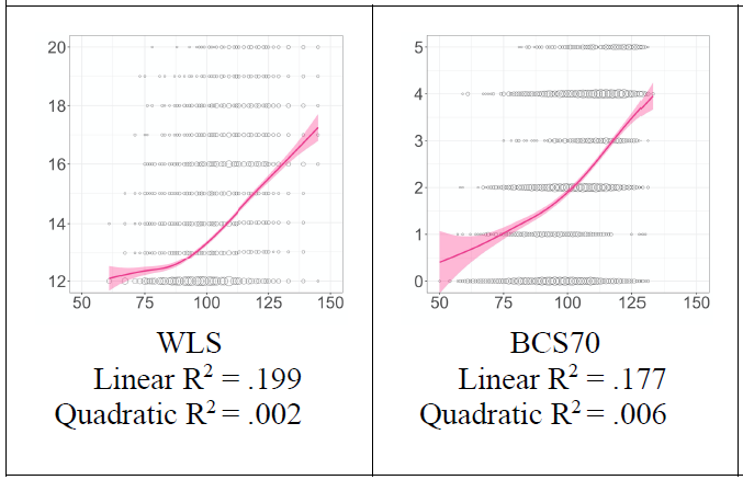
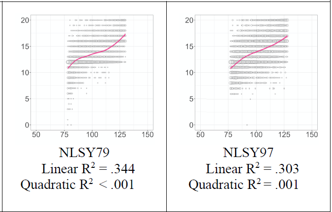
From Figure 5 Brown et al. 2021. “Educational attainment is reported in number of years (WLS, NLSY79, and NLSY97) or using the National Vocational Qualification (NVQ; BCS70).” Bigger circles means the point is weighted more heavily, likely because there are more individuals that achieve that value.
Annual Income
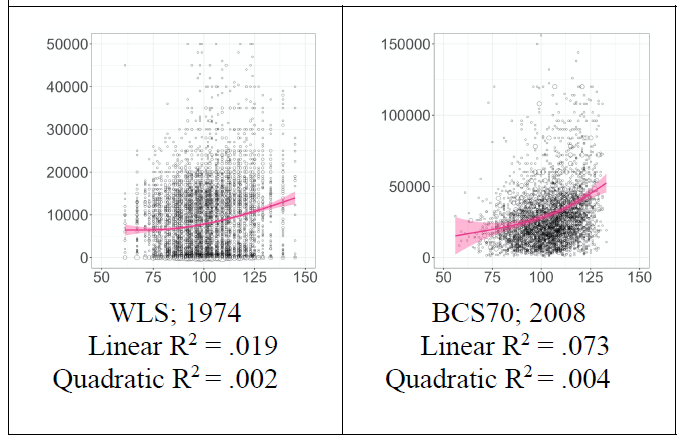
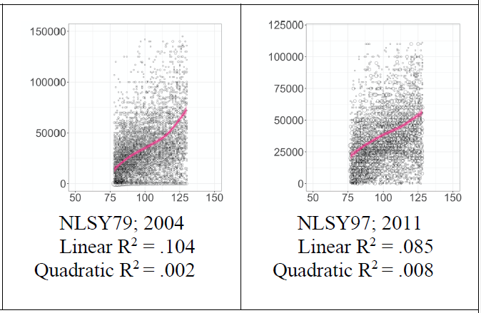
From Figure 5 (Brown et al. 2021). “Annual income is displayed in dollars (or pounds) without a log transformation.”
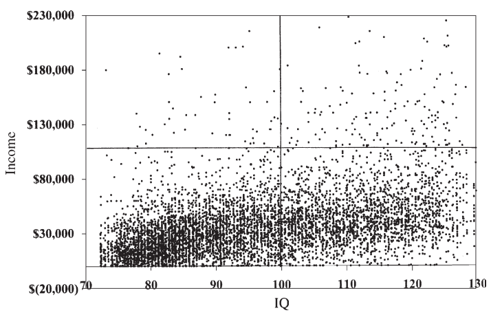
From Fig 1. Zagorsky 2007 (“Do you have to be smart to be rich?”). This uses the NLSY79 data set. r = 0.297
Net Worth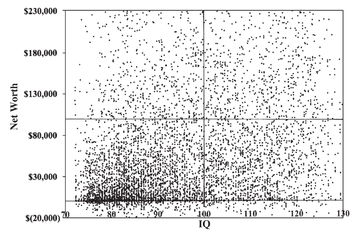
From Fig 2. Zagorsky 2007. This uses the NLSY79 data set. r = 0.156
Job Performance
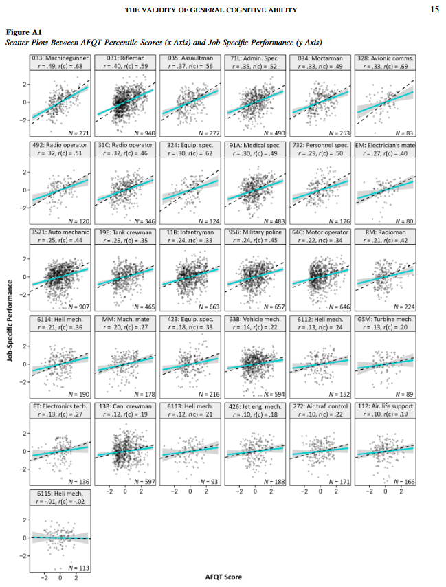
From Hambrick et al. 2024 (“The validity of general cognitive ability”). The graphs appear to depict job performance and AFQT (essentially the Armed Forces IQ test) in terms of standard deviations from the mean, where the mean is 0. N is sample size.
While some slight trends can be seen in these graphs overall, there is large variability for much of the IQ range, showing that whatever predictive utility IQ has for groups, it has little predictive utility for individuals. Even educational attainment—which is what IQ predicts the most strongly—has a fairly wide variation in the data! The lesson is that IQ cannot be used to predict the outcome for an individual. The trend is seen for the group; individuals vary widely.
Indeed, the randomness of the graphs would make one from a hard science background question if the trend for the group is real at all! Certainly, the trend for the group is not that strong. The strength of a correlation between two variables is quantified by r and by squaring r to get R^2. R^2 ranges from 0 to 1, where 1 means a straight line fits the data better and 0 means it fits it worse. In hard sciences like physics, we like R^2 to be bigger than 0.9 for undergraduate labs, though we might accept something like 0.85 depending on how difficult the lab was. We ideally want to see an R^2 of 0.95 or more for these student labs.
By contrast, in social science and psychology, a correlation of 0.5 (R^2 = 0.25) can be considered large (!) (Cohen, J., Statistical power analysis for the behavioral sciences, 1988). Typical values in the social sciences are less than 0.5, as can be seen in the relationships of the graphs posted above. Values of 0.2-0.3 (R^2 = 0.04 to R^2 = 0.09) are very common!
Social scientists do not deny the weakness of the linear fit. Instead, they first make use of R^2 as the proportion of variance explained. This provides a quantitative measure for how much of the variation in a data set that a linear model explains. If R^2 = 0.04, then that means 4% of the variance in the data is explained (https://stats.libretexts.org/Bookshelves/Introductory_Statistics/Introductory_Statistics_(Lane)/19%3A_Effect_Size/19.04%3A_Proportion_of_Variance_Explained).
What does this mean conceptually? Consider one of the plots of Income vs IQ. The individuals in a particular data set differ in their incomes. How much does IQ explain the differences in their incomes? In one of the data sets, we see that R^2 = 0.07. In that data set, IQ explains 7% of the differences, leaving 93% up to other factors. The word explains is intended to be non-causal: changes in IQ are linearly associated with 7% of the variation in income. Equivalently, we can say that IQ linearly predicts 7% of the variation in income, where predict is also understood to state nothing about causality.
Having interpreted R^2 as proportion of variance explained, social scientists than rightly note that humans are very difficult to predict: people are harder to predict than particles! So they continue on to say that if they find a single variable that can explain even 10% of the data, that’s pretty good, considering how unpredictable people are. Indeed, explaining 25% of the data (r = 0.5) is shocking, stunning. They further state that the variables they are measuring are noisy: there is a lot of random noise going on and other causal factors producing the final data point. In other words, IQ is just one part of the story, and if it explains 7% of it, that’s great!
You will see this perspective by one of the authors (Christopher Chabris) in the study Brown et al 2021 study that I linked in the context of defending his results against a critique. He states, “I agree, most of the variance in the outcomes we can and typically measure is not accounted for by general cognitive ability” (https://x.com/cfchabris/status/1882080680336855509). He goes on to defend his results by stating that IQ is nevertheless the best psychological predictor (https://x.com/cfchabris/status/1881520656229253460).
We see then that social scientists are happy to have a weak predictor because it is hard to get anything better when predicting the outcomes of unpredictable people! This is reasonable and all well and good for their field and what they are trying to accomplish: IQ does have some predictive utility for group trends. However, from a hard-science perspective, the numbers are not impressive. From the perspective of the public, they should be aware that IQ has been oversold to them in how much it can predict: because it is a great predictor by the standards of psychology and social science, they speak highly of it, giving a misleading impression to the public of how good it is by a more absolute standard. Just because IQ might be a great predictor by the standards of social science and psychology, does not mean it is a great predictor by the standards of hard science or of the everyday man’s understanding of how the world works.
But there is a deeper problem than the weakness of the correlations. The question is not just how much IQ predicts, but how it predicts—through what causal pathway. If IQ affects income primarily because higher-IQ individuals obtain more education, and education is what employers actually reward, then IQ is not independently driving economic outcomes. Its predictive power for income is operating primarily through educational attainment. This matters regardless of why people differ in how much education they obtain. If income runs through education, then equalizing educational access changes economic outcomes—even if the reason some people currently get more education is partly that they score higher on cognitive tests. The policy-relevant variable is the institutional pathway: who gets access to schooling, for how long, and of what quality. That pathway is amenable to intervention in a way that fixed genetic endowment is not.
A hereditarian will object that the mediation finding itself is uninformative—that it is exactly what we should expect if IQ operates through education. Controlling for education, on this view, is removing the very mechanism through which cognitive ability produces economic value—a textbook causal inference error. The objection is coherent in the abstract. But it rests on a specific empirical premise: that IQ is the fixed upstream cause and education is merely its downstream expression, so that intervening on education without changing IQ would be futile. That premise is false. As we have already seen (in the Environmental Evidence section above), education causally raises IQ by 1–5 points per year of schooling [Ritchie & Tucker-Drob 2018], and a Mendelian randomization study confirmed bidirectional causality of similar magnitude [Anderson et al. 2020]. IQ and education cause each other. The hereditarian cannot treat education as a passive conduit for a fixed cognitive signal when the evidence shows that education actively reshapes the signal itself.
Several independent lines of evidence suggest that education is doing most of the work. Ceci and Henderson, analyzing the Project Talent dataset—a nationally representative sample of over 400,000 high school students first surveyed in 1960—reported that when parental social status and years of schooling were entered as covariates, the effects of IQ as a predictor of adult income were totally eliminated. At the same education level and social class, individuals with low, average, and high IQs earned essentially the same income [Ceci, On Intelligence, Cambridge University Press, 1996, pp. 89–90; citing the Project Talent dataset, originally Flanagan et al. 1960] [verify exact page numbers against the physical book].
Warren, Hauser, and Sheridan (2002), using within-family sibling comparisons in the Wisconsin Longitudinal Study—a design that controls for all shared family background, measured and unmeasured—found that the effects of schooling on occupational standing were far larger than those of cognitive ability throughout the career, though ability showed a small, growing independent effect in later career stages [Warren, Hauser, & Sheridan, “Occupational Stratification Across the Life Course,” American Sociological Review 67 (2002): 432–455]. In a related WLS analysis, Hauser (2010) concluded that “the effects of IQ on economic success are almost entirely mediated by educational attainment” and that “among persons with equal levels of schooling, IQ has little influence on job performance, occupational standing, earnings, or wealth”—including among the self-employed, where credentialism cannot be the explanation [Hauser, “Causes and Consequences of Cognitive Functioning Across the Life Course,” Educational Researcher 39 (2010): 95–109].
A 2025 German longitudinal study (N = 4,387) tracked participants from seventh grade through age 40 and found that once education was included in the model, it mediated virtually all effects of childhood intelligence on income—at every career stage, intelligence’s direct effect on income was statistically indistinguishable from zero [Deutschmann, Becker, & Wu, “Occupational Success Across the Lifespan,” Journal of Intelligence 13, no. 3 (2025): 32]. The authors note that Germany’s highly credential-dependent labor market may amplify education’s mediating role; results could differ in less credential-specific systems like the United States—though the WLS and Project Talent findings, both from the US, show a similar pattern.
Fischer et al. (1996) reanalyzed the same NLSY data Murray used in The Bell Curve with more comprehensive measures of socioeconomic background and found that IQ’s apparent causal power over life outcomes shrank dramatically—an unsurprising result, since Murray measured IQ precisely (a multi-hour test) and SES crudely (three variables at a single time point), virtually guaranteeing that the precisely-measured variable would appear more important [Fischer et al., Inequality by Design: Cracking the Bell Curve Myth, Princeton University Press, 1996]. Genetic evidence points the same direction: Kweon et al. (2024), in a GWAS on income (N = 668,288), found that after statistically removing the genetic variance shared with educational attainment, the residual genetic signal for income had a near-zero genetic correlation with cognitive performance (rg = 0.03). Whatever genetic variants predict income independently of education have essentially nothing to do with cognitive ability [Kweon et al., “Associations Between Common Genetic Variants and Income,” bioRxiv (2024)] [verify whether now published in a peer-reviewed journal].
To be precise about what the evidence warrants: the strongest causal design applied to this question—a Mendelian randomization study by Davies et al. (2019)—found that both intelligence and education have independent positive direct causal effects on household income, suggesting that IQ is not entirely absorbed by education [Davies et al., “Multivariable Two-Sample Mendelian Randomization Estimates of the Effects of Intelligence and Education on Health,” eLife 8 (2019): e43990]. The claim is not that IQ is causally irrelevant. The claim is that IQ’s effect on economic outcomes is largely mediated through education, and that whatever direct effect remains is small. Consider what this means for the hereditarian causal chain: genes → IQ → life outcomes. Even granting the first link (which the genetics section above showed cannot account for more than a few IQ points of group difference), the second link is far weaker than hereditarians suppose. IQ is a weak predictor to begin with (R² ≈ 0.06–0.07 for income). Most of that weak prediction runs through education. And education is shaped by the environment—school quality, family resources, neighborhood conditions—all of which differ dramatically between racial groups in the United States for well-documented historical reasons. The hereditarian needs every link in the chain to be strong. The evidence shows the chain is weak at every point.
Now, what are these correlations of IQ with outcomes in general, aside from the graphs seen above? I will post one table from Brown et al. because it completes the picture when taken with the graphs above, but there is no loss because these are the typical values that one finds. If any are curious, read the following short blog post and some of the references in it for more correlations and considerations (https://developmentalsystem.wordpress.com/2019/11/05/the-predictive-invalidity-of-iq/). Proponents of these IQ tests are especially interested in the correlations with education (usually r = 0.5-0.6), occupational attainment (r = 0.4 or so), job performance (r = 0.5 but has recently been contested to r = 0.31 by Sackett et al. 2022 with confirmation at r = 0.39 by the Hambrick et al. 2024 whose graphs I posted for job-specific performance), and income or wealth (r = 0.2-0.3 or so).
One final note: in some of the graphs, a darker cluster of points can be seen at low IQ range. This has led at least one critique of IQ (Nassim Taleb: https://medium.com/incerto/iq-is-largely-a-pseudoscientific-swindle-f131c101ba39; with a more readable summary by someone else here: https://medium.com/@hyonschu/understanding-nassim-talebs-anti-iq-tweetstorm-dbed194b5e1a) to claim that IQ is better at predicting outcomes at very low IQs (and possibly very high IQs?) but not so great for average outcomes and average IQs. The man writes like a crank and might be one, but this statistical point and potential interpretation of IQ is worth considering. Authors, including Brown et al., dispute the claims of nonlinearity, but there does visually seem to be a clustering at the lower IQ range in the Zagorsky 2007 graphs.
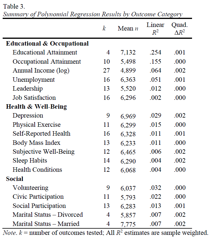
3.14 Crime Statistics
Hereditarians frequently cite crime statistics as evidence for innate moral or behavioral differences between races. The most common formulation, often encountered online, is the claim that Black Americans are 13% of the population but commit 50% of murders. The underlying disparity is real: according to the FBI’s Uniform Crime Reports, Black Americans are arrested for murder at rates several times higher than their share of the population, and this overrepresentation persists for violent crime more broadly. The paper does not deny this. However, statistics are always collected in a context, and any single number can give a misleading picture of what is going on. In this section, I will give a number of other statistics to help fill out that picture and thereby contextualize the disparity better.
Before proceeding, it is worth noting what the hereditarian claim actually is. It is not merely that there is a racial disparity in crime statistics—that much is acknowledged by criminologists of every persuasion. The claim is that this disparity reflects innate, genetically-driven differences in moral character or impulse control between races. That is the inference this section will examine.
3.14.1 The Numbers
The most commonly cited statistic comes from the FBI’s arrest data (Table 43 of the annual Crime in the United States reports). In 2019, approximately 51% of those arrested for murder and nonnegligent manslaughter were Black or African American [FBI UCR, Table 43, 2019]. This is the origin of the “13/50” figure.
However, there is a more comprehensive data source: the FBI’s own Supplementary Homicide Reports (SHR), which track all known murder offenders—not just those arrested, but anyone about whom police have identified any characteristic. When this data is used and the denominator includes offenders whose race is unknown, the proportion of Black offenders is consistently lower: around 36–40% for the years 2010–2020 [FBI, Expanded Homicide Data Table 3, 2010–2020; see also the Bureau of Justice Statistics report on homicide, 2013, p. 7, which explicitly acknowledges the problem of missing offender demographic data]. The year-by-year figures are remarkably stable: 38.2% in 2010, 37.7% in 2011, 37.9% in 2012, 38.0% in 2013, 37.2% in 2014, 36.7% in 2015, 35.9% in 2016, 37.4% in 2017, 38.7% in 2018, 39.6% in 2019, and 38.8% in 2020 [compiled from FBI Expanded Homicide Data Table 3 for each year; verify against original tables]. The “50%” figure is obtained by looking only at arrestees and excluding unknowns from the denominator. The “38%” figure is obtained by looking at all known offenders and including unknowns. Neither tells us about the roughly 40% of homicides that are never solved at all: the average annual homicide clearance rate is approximately 60%, meaning that a large fraction of offenders are entirely unidentified [FBI UCR clearance data; BJS, 2013]. The true racial distribution of all murder offenders is genuinely uncertain. What can be said is that the commonly cited figure is the highest of several defensible estimates from the FBI’s own data.
[FLAG: I would like to compile multi-year data for both the arrest figures (Table 43) and the SHR known-offender figures (Table 3), including years after 2019 (2020–2023), to present averages and trends. This may require downloading FBI Excel files. If time does not permit, the 2010–2020 SHR data above and the 2019 arrest figure will suffice, but a broader range would be more robust.]
For violent crime more broadly—murder, rape, robbery, and aggravated assault combined—the disparity is smaller. In 2019, approximately 27% of those arrested for violent crimes were Black [FBI UCR, Table 43, 2019]. This is still disproportionate relative to the 13.4% population share, but it is not “50%.” The “13/50” formulation applies only to murder arrests, not to violent crime in general and not to crime as a whole.
One category worth noting is rape, where the disparity is smaller still. In 2019, approximately 67% of those arrested for rape were White and 27% were Black [FBI UCR, Table 43, 2019]—an overrepresentation of roughly 2× for Black Americans, far less dramatic than the 4–6× overrepresentation for murder.
A note on the data: the FBI’s UCR program classifies most Hispanics (approximately 93%) as “White” for purposes of the race variable [ACLU; see also the Wikipedia summary of the UCR classification system]. This means the “White” arrest figures are inflated relative to the non-Hispanic White population, and the true non-Hispanic White arrest rate is somewhat lower than reported. Hereditarians sometimes point this out to argue the real Black–White gap is even wider. This is likely true to some degree for murder, though the magnitude is hard to quantify because the ethnicity variable in the FBI data is severely underreported (roughly 55% of offenders in the SHR have unknown ethnicity) [FBI SHR data documentation]. The same classification issue also affects crime categories where whites are overrepresented, such as DUI and liquor offenses, so it is not a one-directional correction.
3.14.2 Who Is Actually Committing These Crimes?
Consider what the numbers mean in terms of the actual people involved. In 2019, approximately 4,800–5,000 Black individuals were arrested for murder [calculated from FBI Table 43, 2019]. The Black population of the United States was approximately 44 million. That is roughly 0.011%—about one one-hundredth of one percent—of the Black population arrested for murder in a given year. Even after accounting for unsolved cases by assuming the unknowns distribute proportionally, the figure might rise to 0.015–0.02%. Under any plausible assumptions about cumulative lifetime risk, well under 1% of Black males will ever commit a homicide [see BJS and related analyses; this is a rough estimate and should be treated as such].
For all violent crime combined, approximately 132,000 Black individuals were arrested in 2019 [FBI Table 43, 2019]. That is approximately 0.30% of the Black population. Over 99.7% of Black Americans were not arrested for any violent crime that year.
These figures are for violent crime specifically. If one expands the frame to include all arrests—drug possession, property crime, DUI, disorderly conduct, simple assault, and everything else the FBI tracks—the numbers are larger. In 2019, the FBI estimated 10.1 million total arrests nationwide, excluding traffic violations [FBI, Crime in the United States, 2019]. Black Americans accounted for 26.6% of these, or roughly 2.7 million arrest events, which is approximately 6% of the Black population. For non-Hispanic White Americans, the comparable figure is roughly 3.5–4.5% [calculated from 69.4% of 10.1 million arrests divided by the non-Hispanic White population of approximately 197 million]. But this all-offenses figure is dominated by non-violent categories: drug possession alone was the single largest arrest category in 2019 at 1.35 million, followed by property crime, simple assault, and DUI at roughly one million each; violent crime accounted for under 500,000 of the 10.1 million total, less than 5% [FBI, Persons Arrested, 2019]. The all-offenses figure also dropped substantially over the preceding decade—from roughly 8–9% to roughly 6% for Black Americans—as total arrests nationwide fell from 13.1 million in 2010 to 10.1 million in 2019 [FBI, Crime in the United States, 2010 and 2019]. The violent-crime figures above are the relevant ones for the hereditarian claim about violent behavior, and those are the figures this section uses.
Furthermore, the offending population is heavily concentrated by sex and age. Approximately 88% of those arrested for murder are male [FBI Table 42, 2019]. The offenders are overwhelmingly young men between the ages of 18 and 30. The number of people generating these statistics is a small subset of a small subset of the Black population: young men, in specific circumstances, in specific places. To attribute their behavior to 44 million people spanning every region, class, age, and sex is not a conclusion that the statistics support.
It is also worth noting that arrest counts are not counts of unique individuals. A single person arrested multiple times in a year generates multiple entries in the arrest data. A small number of high-frequency repeat offenders can therefore generate a disproportionate share of the total arrests. The already-small fraction of the Black population involved in violent crime is further compressed by this: the statistics are partly driven by an even smaller group of repeat offenders cycling through the system [see the general criminological literature on the concentration of offending among a small number of individuals; specific race-disaggregated recidivism data for homicide is limited, so I flag this for further sourcing before publication].
3.14.3 What Do We Know About Wrongful Convictions?
Some fraction of the Black crime statistics includes people who did not commit the crime they were convicted of. The National Registry of Exonerations, a joint project of the University of California Irvine, the University of Michigan Law School, and Michigan State University College of Law, has tracked wrongful convictions since 1989. Their 2022 report found that Black Americans are 13.6% of the population but account for 53% of all exonerations [Gross et al., Race and Wrongful Convictions in the United States, 2022]. In 2023, 61% of exonerees were Black; in 2024, 60% [National Registry of Exonerations Annual Reports, 2023 and 2024].
For murder specifically, the report found that Black defendants convicted of murder are approximately 50% more likely to be innocent than other convicted murderers. The convictions of Black murder defendants were also substantially more likely to involve police misconduct: 58% of Black murder exonerees faced police misconduct, compared to 38% of White murder exonerees [Gross et al., 2022]. For drug crimes, the disparity is even starker: Black Americans are approximately 19 times more likely to be wrongfully convicted of drug offenses, despite similar drug use rates across racial groups [Gross et al., 2022].
This does not eliminate the disparity—even after correction, Black Americans would still be overrepresented among homicide offenders. But it demonstrates that the official statistics systematically overcount Black offending. The correction is not trivial, and the pattern has been confirmed across more than three decades of data.
3.14.4 Felony Convictions
Some will object that per-year figures understate the scope of the problem. A study published in Demography estimated that as of 2010, approximately 33% of Black adult males in the United States had a felony conviction, compared to roughly 13% of adult males overall [Shannon et al., “The Growth, Scope, and Spatial Distribution of People With Felony Records in the United States, 1948–2010,” Demography 54, no. 5 (2017): 1795–1818]. That is a real and sobering figure, and this paper will not minimize it. But several facts are essential to understanding what it means.
First, “felony” is a legal category whose boundaries are set by legislators, not by nature. It encompasses everything from marijuana possession to murder, depending on jurisdiction. Drug offenses accounted for roughly a quarter of state prison admissions in 2019, and many felony convictions result in probation rather than prison time at all [Pew Charitable Trusts, “Drug Arrests Stayed High Even as Imprisonment Fell From 2009 to 2019,” 2022]. The 33% figure is not “33% of Black males have committed a violent crime.” It is “33% have been convicted of something a legislature classified as a felony”—a category that expanded dramatically during the era of mass incarceration.
Second, the growth trajectory is itself evidence against a genetic explanation. The figure rose from 13.3% in 1980 to 33% in 2010—a near-tripling in three decades that Shannon et al. explicitly situate within what they call a “historic increase in criminal punishment,” including mandatory minimum sentencing, three-strikes laws, and the War on Drugs [Shannon et al., 2017]. The bipartisan First Step Act of 2018 acknowledged that many of these policies were excessive, and incarceration rates have been declining since their peak. If felony conviction rates were primarily a reflection of innate racial tendencies, they would not triple in thirty years because Congress changed the sentencing guidelines.
Third, the wrongful conviction evidence presented above applies to felony convictions generally, not only to homicide. Black Americans are seven times more likely to be falsely convicted of serious crimes overall, and nineteen times more likely for drug crimes specifically [Gross et al., 2022]. Some unknown but non-trivial fraction of the 33% figure consists of people who should not have been convicted. The NRE has also documented systematic police fabrication of drug evidence against Black defendants in multiple cities, including Chicago, Philadelphia, and New York [Gross et al., 2022]. These are not marginal corrections; they represent thousands of convictions across decades.
3.14.5 Crime Is Concentrated in Specific Neighborhoods
One of the most important contextual facts about violent crime is that it is geographically hyper-concentrated. Research consistently shows that a tiny fraction of locations accounts for a vastly disproportionate share of violence. In Boston, 74% of crimes occurred in just 5% of city blocks between 1980 and 2008 [Braga et al., 2010]. Across cities, roughly 1% of street segments typically account for 25% of crime, and 5% of neighborhoods account for approximately 50% of homicides [Braga et al., 2010; Weisburd et al., 2004; see also the OpenCrime analysis of geographic concentration].
The variation within a single city can be staggering. In Chicago in 2019, the most dangerous neighborhood (West Garfield Park) had a homicide rate of 131 per 100,000. The 28 safest neighborhoods in the same city had rates under 2 per 100,000, and many had zero homicides [data cited in Manhattan Contrarian analysis of Chicago neighborhoods]. The United States overall that year had a rate of about 5 per 100,000.
As a Brookings Institution analysis put it: “The vast majority of people who live in neighborhoods with concentrated poverty are not involved in violent crime. Only a very small number of residents in these areas commit homicides, and they are quite different from their neighbors” [Brookings, 2024]. Those residents are disproportionately male, under 30, high school dropouts, and unemployed—the same Brookings analysis notes that approximately 40% of people incarcerated in U.S. prisons did not graduate from high school or earn a GED, compared to about 9% of all adults, and that males under 30 commit more than half of all murders [Brookings, 2024].
The implications for racial attribution are direct. Black Americans living in suburban communities, rural areas, or middle-class urban neighborhoods do not experience or perpetrate elevated violent crime. The violence is concentrated in specific blocks of specific cities, characterized by concentrated poverty, family disruption, abandoned infrastructure, and limited economic opportunity. If the racial disparity in crime were driven by innate genetic differences, we would expect it to be roughly constant across environments—appearing wherever Black Americans live, at approximately the same magnitude. Instead, the magnitude varies enormously with neighborhood conditions: from staggering in concentrated-poverty neighborhoods to negligible in low-poverty areas (as the Sampson and Chetty findings below will confirm). This is the signature of an environmental cause, not a genetic one. To take statistics generated by a few thousand individuals in these specific locations and attribute them to the nature of 44 million people across every class, region, and context is a statistical error of the first order.
3.14.6 Structural Factors Explain Most or All of the Gap - AI gen (Verify)
If the racial disparity in violent crime is not driven by innate differences, what does explain it? The criminological literature provides a strong answer: structural and neighborhood-level factors.
Robert Sampson and colleagues (2005), in a landmark study published in the American Journal of Public Health, analyzed 2,974 individuals across 180 Chicago neighborhoods over seven years. They found that before controlling for any factors, the odds of perpetrating violence were 85% higher for Black participants compared to White participants. But after accounting for parental marital status, immigrant generation, and dimensions of neighborhood social context, over 60% of the Black-White gap was explained. The entire Latino-White gap was explained [Sampson, Morenoff, & Raudenbush, 2005]. Using the nationally representative National Longitudinal Survey of Adolescent Health, Bellair and McNulty (2005) went further: they found that concentrated disadvantage explained the entire Black-White gap in self-reported serious violence. Notably, indicators of verbal ability and academic achievement were less potent than community-level disadvantage in explaining racial differences in violent behavior [Bellair & McNulty, 2005; see also the National Academies review, Reducing Racial Inequality in Crime and Justice, 2023].
Some hereditarians argue that the racial disparity persists even after controlling for income, citing research showing that Black men raised in high-income families still have higher incarceration rates than White men raised in low-income families. This claim appears to draw on the important work of Chetty et al. (2020), who documented exactly that pattern. But Chetty also found that this pattern was not true for Black women, and—crucially—was driven by neighborhood characteristics, not by race per se. Black boys raised in low-poverty neighborhoods did not show the elevated incarceration pattern. The finding supports a neighborhood-effects explanation, not a genetic one [Chetty et al., 2020; this is the same study cited earlier in this paper regarding IQ and neighborhood effects].
3.14.7 The Great Crime Decline - (Verify)
Perhaps the single strongest argument against a genetic explanation for the racial crime disparity is the speed at which crime rates change. Between the early 1990s and the mid-2000s, violent crime in the United States fell by more than 50%. The Black homicide rate fell even more steeply—unsurprisingly, since the crack epidemic of the late 1980s had hit Black communities hardest, and its end brought the greatest relief to those same communities.
The evidence from individual cities is dramatic. In five New York City police precincts that were over 80% Black and had high poverty rates—including Harlem and Brooklyn’s Bedford-Stuyvesant—murder rates dropped 78% between 1990 and 2000, exceeding the citywide decline of 73%. The neighborhoods stayed Black. They stayed poor. The crime rate nevertheless dropped by more than three-quarters in a single decade [data from Claremont Review of Books analysis of NYPD precinct data].
Genetic change operates on generational timescales. Allele frequencies across a population of 44 million people do not shift appreciably in ten years. A 50–78% decline in homicide rates within a single decade—and the dramatic year-to-year fluctuations visible in the FBI’s own data across the decades—is not compatible with a genetic explanation. If violent crime were primarily genetic, the rate would be approximately stable across decades within the same population. It is not. It fluctuates in response to the crack epidemic, the end of the crack epidemic, policing changes, the COVID-19 disruption, and other environmental factors. This is the same argument, applied to crime, that the Flynn Effect provides for IQ: the rate of change is too fast for genetics.
[FLAG: Verify the NYC precinct-level data against original NYPD records. The Claremont Review of Books analysis is a secondary source.]
3.14.8 Where Whites Are Overrepresented
If overrepresentation in crime statistics is evidence of racial nature, the logic should be applied consistently. But it is not. There are several categories in which White Americans are overrepresented relative to their population share, and no one attributes these to innate racial character.
Suicide. The non-Hispanic White suicide rate in 2023 was 17.6 per 100,000, compared to approximately 8.5 for non-Hispanic Black Americans. White males specifically had a rate of 28.0 per 100,000. White people accounted for 75% of all 49,316 suicide deaths in 2023. Suicide kills more than twice as many Americans each year as homicide (49,316 versus 22,830 in 2023) [CDC, WISQARS, 2023; NIMH suicide statistics, 2023; verify that “non-Hispanic” applies to the 8.5 Black figure].
DUI and alcohol offenses. According to FBI data, Black youth are overrepresented in all juvenile offense categories except DUI, liquor law violations, and drunkenness—meaning White youth are disproportionately represented in those categories [FBI UCR, 2008, as reported in the Race and Crime Wikipedia summary; verify against original Table 43].
White-collar crime. Academic research has documented that White Americans are overrepresented in elite white-collar crime, including corporate fraud, securities violations, and organizational crime [Sohoni & Rorie, 2021]. Annual losses from white-collar crime are estimated at $426 billion to $1.7 trillion—dwarfing the economic costs of street crime by orders of magnitude [Zippia white-collar crime statistics; verify primary source].
The rhetorical question writes itself. If Black overrepresentation in homicide statistics is evidence of innate Black moral deficiency, is White overrepresentation in suicide evidence of innate White despair? Is the opioid epidemic—which disproportionately devastated White rural communities—evidence of innate White susceptibility to addiction? Is elite corporate fraud evidence of innate White dishonesty? No hereditarian would accept these inferences. Yet the logic is identical. The consistent alternative explanation is that different populations facing different structural conditions manifest different pathologies. The opioid crisis struck White rural communities not because of White genetics but because of pharmaceutical marketing, economic decline, and cultural isolation. Violence is concentrated in specific Black urban neighborhoods not because of Black genetics but because of concentrated poverty, family disruption, and structural disadvantage. Both are real problems. Neither is a racial nature.
3.14.9 On Attributing Tendencies to Groups
There is a legitimate question about when it is appropriate to say that a group has a tendency toward something. The Bible itself does this: Paul quotes a Cretan prophet saying “Cretans are always liars, evil beasts, lazy gluttons” and affirms “this testimony is true” (Titus 1:12–13). The prophets attribute national sins to Israel as a people. It is not illegitimate to observe that specific communities face specific problems.
But there is an essential distinction between two kinds of claims. The first: specific communities, shaped by specific historical and structural conditions, manifest specific problems—a sociological observation directed at understanding and remedying those conditions. The second: this race has an innate tendency toward this behavior—a biological claim directed at establishing a hierarchy. The Bible always operates in the first mode. The prophets attribute sins to Israel to call them to repentance, never to establish the permanent moral superiority of another nation. The attribution is cultural and moral, not biological; it is provisional (cultures change; Israel was called to change), not permanent; and it is directed at the group’s good, not at justifying the dominance of another group.
The crime statistics we have examined in this section are consistent with the first kind of claim. There are specific communities in the United States—concentrated in specific neighborhoods of specific cities, characterized by specific structural conditions—where violent crime rates are high. These communities are disproportionately Black, for historical reasons that are themselves well-understood (the legacy of segregation, redlining, and economic exclusion that created the concentrated-poverty neighborhoods in the first place). Recognizing this as a real problem is not the error. The error is the leap from a community-level problem driven by specific conditions to a racial nature attributed to 44 million people, the vast majority of whom do not live in those neighborhoods, do not commit violent crimes, and share nothing with the offending population except the color of their skin. This leap is not supported by the crime statistics. It is not supported by the criminological literature. It is not supported by the temporal evidence (crime rates change too fast for genetics). And it is not supported by the geographic evidence (if it were racial nature, it would manifest everywhere, not only on specific blocks of specific cities). Some scientific racists have invoked the Titus passage to justify attributing besetting sins to an entire race, but the passage concerns a single, culturally homogeneous island—not a continental-scale racial group of 44 million people spanning every region, class, and cultural context in America. The application does not follow.
3.14.10 The Base-Rate Problem: Why Discrimination Does Not Follow
Even using the highest arrest-based figures and granting the disparity as real (as we have throughout this section), the statistics do not support the practical inference that one should treat individual Black people with suspicion. For murder: the probability that a randomly encountered Black person is a murderer in a given year is approximately 0.01–0.02%. For every 10,000 Black individuals one encounters, at most one or two have committed a homicide. The false-positive rate of treating Black individuals as dangerous on the basis of murder statistics is over 99.98%.
For violent crime more broadly, the numbers are larger but the conclusion is the same. Approximately 0.30% of the Black population was arrested for any violent crime in 2019. That means 99.7% were not. For White Americans (including Hispanics per UCR classification), approximately 0.12% were arrested for violent crime. Both base rates are small; both populations are overwhelmingly non-violent.
This is a textbook instance of confusing properties of a distribution with properties of an individual. Even where a group average differs from another group’s average, the overlap between the two distributions is enormous, and the base rate for the behavior in question is vanishingly small in both groups.
Why, then, does the association between race and violent crime feel so compelling despite these numbers? Part of the answer lies in how human language and cognition handle group-level claims about dangerous properties. Research in philosophy of language has shown that generic statements—statements of the form “Xs are Y,” without a quantifier—operate with dramatically different thresholds depending on whether the attributed property is dangerous or mundane. “Mosquitoes carry malaria” is accepted as true even though only a small fraction of mosquitoes carry the parasite. “Americans are left-handed” feels false even though roughly 10% are—far more than the fraction of mosquitoes carrying malaria. The difference is that dangerous or frightening properties trigger a cognitive threshold so low that even vanishingly rare prevalence is sufficient for the generic to feel true [Leslie, “The Original Sin of Cognition: Fear, Prejudice, and Generalization,” Journal of Philosophy 114, no. 8 (2017): 393–421]. The same machinery is at work when someone hears “Black people commit murder” and finds it compelling: the property is frightening, so the cognitive threshold drops to near zero, and a 0.01% base rate is enough to sustain the generalization. This is not a matter of the listener being stupid or malicious. It is a structural feature of how generic sentences work in human cognition. Recognizing this helps explain why the base-rate math presented above is necessary: it corrects for a built-in bias in how we process group-level claims about danger.
Moreover, once one conditions on location and circumstance—which is what any rational risk assessment does—race adds almost no predictive information. As the neighborhood concentration evidence above demonstrates, crime clusters in specific blocks with specific structural conditions, not across racial populations as a whole. A Black professional in suburban Raleigh lives in a neighborhood with the same low crime rate as his White neighbor’s. The relevant question is always about the specific circumstances (neighborhood, time of day, situation), not about the race of the person one encounters. A comparison may help make the point: the non-Hispanic White male suicide rate is approximately 28 per 100,000 per year, which is roughly 0.028%. The probability that a randomly encountered Black person is a murderer is approximately 0.01–0.02% per year. By the logic of racial profiling, one has roughly two to three times more statistical reason to worry that a White man will kill himself than that a Black man will kill you. No one would suggest treating White men with preemptive suspicion on the basis of suicide statistics, because the base rate is obviously too low to warrant it. The same reasoning applies to crime statistics, and for the same reason.
[Table or figure suggestion: A comparison table showing the base rates side-by-side: “Annual probability that a random Black individual is a murder offender: ~0.01–0.02%”; “Annual probability that a random White male commits suicide: ~0.028%”; “Annual probability that a random White individual is arrested for DUI: [calculate]”. This would visually drive home the base-rate point.]
4 African History
The hereditarian picture of sub-Saharan Africa is one of permanent civilizational absence.82 Murray treats Africa’s history as a puzzle requiring genetic explanation; the online HBD community is less careful, routinely asserting that sub-Saharan Africa never produced literate, urbanized, or politically complex societies. This claim is historically false, and it also turns out that early Europeans had a positive view of the African peoples. We will briefly dispatch these claims in this section.
Before turning to the historical record, it is worth noting that Scripture itself identifies Egypt as “the land of Ham” (Ps. 105:23, 27; 106:22)—not once, but repeatedly, across multiple psalms. The Hamitic genealogy also produces Nimrod, whom Genesis 10 identifies as the world’s first empire-builder (vv. 8–12). The hereditarian attempt to exclude Egypt and the ancient Near East from Africa’s civilizational record requires erasing a biblical identification that the biblical authors never thought to obscure. Moreover, Scripture attributes the decline of nations—Egypt, Assyria, Israel itself—to divine judgment for specific sins (Isa. 19; Ezek. 29–32), the same framework applied across all nations. Nothing in the biblical text suggests that such judgment takes the form of permanent cognitive degradation of any lineage.
It is also worth confronting the popular assumption that Ham settled Africa, Shem the Middle East, and Japheth Europe. This is not what Genesis says. As we saw earlier in the common-sense section, Carter has documented that the Table of Nations shows massive geographic overlap among the descendants of all three sons—Ham’s line reaching into Anatolia, Canaan, Mesopotamia, and Arabia alongside Shem’s and Japheth’s—and the Bible says nothing specific about who settled sub-Saharan Africa [Carter, “Can we place the sons of Noah on the Y chromosome tree?”, creation.com, 2024; see the figure above in the common-sense section].83 The equation of Ham with sub-Saharan Africa and all its people is an imposition on the text, not a reading derived from it.
4.1 Ancient African Civilizations — A Brief Overview
Here is a brief historical survey of African civilizations that demonstrates that the hereditarian premise does not survive contact with the actual record.
The Mali Empire. At its height in the 13th and 14th centuries, the Mali Empire was one of the wealthiest polities on earth. Its most famous ruler, Mansa Musa, undertook a pilgrimage to Mecca in 1324 with a caravan so lavishly provisioned with gold that his spending in Cairo reportedly depressed the gold market for a decade afterward. Contemporary Arab chroniclers documented this; it is not legend [al-Umari, Masalik al-Absar, 14th c.; see Levtzion and Hopkins, Corpus of Early Arabic Sources for West African History, 2000]. The city of Timbuktu, within the empire and later the Songhai successor state, was a major center of Islamic learning and manuscript culture. The University of Sankore attracted scholars from across the Islamic world. Thousands of manuscripts from this intellectual tradition survive today — legal texts, astronomical works, theological treatises, medical texts — and are the subject of ongoing preservation efforts [Hunwick, Timbuktu and the Songhay Empire, 2003; the Timbuktu Manuscripts Project]. This is not a civilization that lacked intellectual culture.
[Image: Mansa Musa depicted in the Catalan Atlas of 1375, holding a gold nugget — one of the earliest European depictions of a sub-Saharan African ruler]
Great Zimbabwe. In southeastern Africa, the stone ruins of Great Zimbabwe stand as the remains of a city that was the center of a major trading empire from roughly the 11th to 15th centuries. The Great Enclosure wall stands over 30 feet high and extends more than 800 feet, built of cut granite blocks fitted together without mortar. The site was a hub for trade in gold, ivory, and cattle, with links reaching to the Swahili coast and, through it, to the Indian Ocean trade network [Pikirayi, The Zimbabwe Culture, 2001; Connah, African Civilizations, 3rd ed., 2015].
The historiographical footnote here is telling: when European colonists first encountered Great Zimbabwe in the late 19th century, they refused to believe Africans had built it. Theories attributing it to Phoenicians, Arabs, or the Queen of Sheba’s kingdom circulated for decades. Archaeological investigation has conclusively established that it was built by the ancestors of the Shona people [Pikirayi 2001; see also Fontein, The Silence of Great Zimbabwe, 2006 — verify]. The refusal to credit African builders is itself a case study in the bias this paper addresses.
[Image: The Great Enclosure at Great Zimbabwe, showing the dry-stone wall construction]
The Kingdom of Aksum (Ethiopia/Eritrea). Aksum was a major power in the ancient world from roughly the 1st through the 7th centuries AD, controlling territory in modern Ethiopia, Eritrea, and at times Yemen. The Persian prophet Mani (3rd century) listed Aksum alongside Rome, Persia, and China as one of the four great empires of the world [Munro-Hay, Aksum: An African Civilisation of Late Antiquity, 1991; verify Mani quote]. Ethiopia appears in Scripture over 37 times, and the Queen of Sheba’s visit to Solomon (1 Kings 10; 2 Chronicles 9) — whom Ethiopian tradition identifies as Queen Makeda — ties Ethiopian history to the Solomonic narrative. The Ethiopian eunuch baptized by Philip in Acts 8:26–39 is one of the earliest recorded conversions of a Gentile. King Ezana of Aksum adopted Christianity as the state religion around 340 AD, roughly concurrent with Constantine, making Aksum one of the earliest Christian kingdoms in the world [Munro-Hay 1991; Phillipson, Foundations of an African Civilisation, 2012]. The Ethiopian church has maintained an unbroken Christian tradition from the 4th century to the present day.
Ethiopia is also the only African nation that successfully resisted European colonization during the Scramble for Africa.84 When Italy attempted to colonize Ethiopia in 1896, Emperor Menelik II mobilized an army of over 100,000 and decisively defeated the Italian force at the Battle of Adwa. The victory was so complete that Italy was forced to recognize Ethiopian sovereignty outright — a result that stunned European powers accustomed to viewing Africans as incapable of organized military resistance. As one historian noted, the Ethiopian victory at Adwa directly challenged the European doctrines of racial superiority that undergirded the colonial project [see Marcus, A History of Ethiopia, 2002 — verify; see also Jonas, The Battle of Adwa, 2011 — verify]. Mussolini later invaded in 1935 partly to avenge this humiliation, and required the use of mustard gas — a banned chemical weapon — to succeed. Ethiopia was liberated in 1941.
[Image: One of the Aksumite stelae at Aksum, showing the architectural sophistication of the kingdom]
The Kingdom of Benin. The Kingdom of Benin (in modern-day Nigeria, not the modern nation of Benin) was a sophisticated polity known for its political organization, extensive trade networks, and extraordinary artistic production. The Benin Bronzes — intricate cast brass and bronze plaques and sculptures depicting court life, history, and ritual — are among the finest metalwork produced anywhere in the premodern world. They are now one of the most contested bodies of African art, since most were looted by the British in the 1897 punitive expedition [Connah 2015]. Hereditarians have used Benin’s later-period practices of human sacrifice and participation in the slave trade as a negative example, but this argument receives fuller treatment in its own section below, where I examine what early European visitors actually recorded about Benin City before colonial-era ideology shaped the narrative.
[Image: A Benin Bronze plaque showing a court scene — examples are held in the British Museum, Metropolitan Museum of Art, and other institutions]
The Kingdom of Kongo. The Kingdom of Kongo, centered in what is now the western Democratic Republic of Congo, Republic of Congo, and northern Angola, was a centralized state with a sophisticated political structure when the Portuguese first made contact in 1483. The kingdom had a system of provincial governors, tax collection, a judicial system, and a capital city at Mbanza Kongo with a population estimated in the tens of thousands [Thornton, Africa and Africans in the Making of the Atlantic World, 1998; see also Hilton, The Kingdom of Kongo, 1985 — verify]. Upon Portuguese contact, King Nzinga a Nkuwu converted to Christianity and was baptized as João I in 1491. His son Afonso I (Mvemba a Nzinga), who ruled from approximately 1509 to 1543, was literate in Portuguese and conducted a sustained diplomatic correspondence with the Portuguese crown — letters that survive today and are among the most remarkable documents in African history. In these letters, Afonso protested the abuses of the slave trade, requested teachers and craftsmen, and sought to modernize his kingdom along Christian lines [Thornton 1998; see also Heywood and Thornton, Central Africans, Atlantic Creoles, and the Foundation of the Americas, 1585–1660, 2007 — verify].
The contrast between the Kingdom of Kongo at Portuguese contact and the condition of the modern Democratic Republic of Congo is stark, and worth noting precisely because hereditarians tend to treat Africa’s present difficulties as evidence of permanent incapacity. The DRC’s modern troubles have specific historical causes — the catastrophic exploitation under Leopold II’s Congo Free State, subsequent Belgian colonial mismanagement, Cold War interference, and the ongoing resource extraction that funds regional conflict [find citation] — none of which are genetic. A kingdom that produced literate Christian rulers conducting diplomacy with European powers in the 16th century does not fit the hereditarian narrative of civilizational absence.
[Image: A letter from King Afonso I of Kongo to the King of Portugal, or alternatively, a map showing the extent of the Kingdom of Kongo at its height]
These are not exhaustive examples. I have not discussed Jenne-jeno, one of the oldest known cities in sub-Saharan Africa, with urban settlement from roughly 250 BC [McIntosh, Ancient Middle Niger, 2005 — verify]. I have not discussed the Swahili coast city-states, or the Kingdom of Kush, or the Nok culture’s terracotta sculptures. The point is not to be exhaustive but to establish a simple fact: the hereditarian premise that sub-Saharan Africa has always been without civilization is historically false.
For a comprehensive archaeological overview, see Graham Connah, African Civilizations: An Archaeological Perspective, 3rd ed. (Cambridge UP, 2015), which surveys urbanism, state formation, and technology across the continent. For the reader who wants to go further, John Thornton’s Africa and Africans in the Making of the Atlantic World, 1400–1800, 2nd ed. (Cambridge UP, 1998) is the standard text on African polities in the early modern period. Importantly, both Connah and Thornton work from archaeological evidence and primary documentary sources — their conclusions do not depend on any particular account of deep prehistory and are compatible with a creationist framework.
The archaeological record and IQ. There is one more point to make here, and it connects African history back to the IQ discussion. The hereditarian psychologist J. Philippe Rushton not only claimed that African populations suffer from severe cognitive deficits compared to other modern humans, but placed these claimed deficits in a prehistorical context, arguing that such differences have existed as long as the populations themselves have been distinct. If this claim were true — if African populations had been operating with substantially lower cognitive capacity for thousands of years — this should be detectable in the archaeological record. Cognitive capacity shows up in material culture: tool complexity, symbolic behavior, trade network organization, architectural planning, and artistic production all require the very capacities Rushton claims were deficient.
Archaeologist Scott MacEachern tested exactly this claim. In his paper “Africanist Archaeology and Ancient IQ” (World Archaeology 38(1), 2006), MacEachern examined the archaeological record of sub-Saharan Africa against the predictions of the hereditarian cognitive-deficit model. His finding was straightforward: the archaeological record does not support the claims made by these researchers. The development of complex societies, urbanization, long-distance trade, metallurgy, and symbolic culture across sub-Saharan Africa followed trajectories comparable to those on other continents, emerging according to their own internal logics and in response to local conditions [MacEachern 2006, pp. 72–92].
A hereditarian might respond: but some of these developments occurred later in Africa than elsewhere — doesn’t that require explanation? MacEachern addresses this honestly. He concedes, for example, that African plant domestication is “certainly later than was the case in many other areas of the world.” But he also notes that the variety of indigenous African plant domesticates is comparable to those from the Near East and probably exceeds the diversity of East Asian and American domesticates — and animal domestication in the Sahara and Sahel dates to the eighth millennium BP, quite early by any standard. More fundamentally, the hereditarian claim is not that Africa developed slightly later [confirm slightly later] in some areas. The claim is that African populations suffer from severe cognitive deficits — borderline mental retardation, an average IQ of 70 — that have persisted over evolutionary timescales. The archaeological record of the civilizations surveyed above is flatly inconsistent with that claim. Timing differences in specific domains have well-understood ecological and geographical explanations that do not require positing cognitive deficiency — and it is worth noting that Europe itself was a latecomer in agriculture, receiving its domesticates from the Near East rather than developing them independently.
MacEachern also drew a parallel that deserves emphasis: the Flynn Effect. Taken at face value, the Flynn Effect implies that the average North American adult living around a century ago would have scored approximately IQ 75 on modern tests — a value closely comparable to those derived for twentieth-century African populations by Rushton and Lynn. This is, as MacEachern observes, a nonsensical result — and even Herrnstein and Murray, the authors of The Bell Curve, acknowledged as much, writing that when one looks at the science, literature, politics, and arts of previous generations, one does not get the impression of diminished intellect [Herrnstein and Murray 1994, pp. 308–9; cited in MacEachern 2006, p. 84]. MacEachern’s observation is pointed: if we rightly refuse to believe our great-grandparents were cognitively deficient on the basis of what they actually accomplished, we should apply the same standard to African populations — and the archaeological record shows that they pass it.
This point complements what we have already seen in the genetics section. The genetic evidence shows that the observed between-population variation on cognitive-relevant loci is expected to be small and is consistent with drift; the archaeological evidence shows that the behavioral record — the record of what people actually did and built — does not look like the record of a population laboring under severe cognitive deficits. These are independent lines of evidence converging on the same conclusion.
4.2 Portuguese Views — The First European Witnesses
The civilizations surveyed above are not the only evidence against the hereditarian premise. There is another line of testimony that deserves attention, precisely because of who is doing the testifying: the earliest European visitors to sub-Saharan Africa themselves.
The Portuguese were the first sustained European presence in sub-Saharan Africa, beginning in the mid-15th century and continuing through the 17th. This matters for our purposes because these accounts predate the systematic racial ideology that shaped European descriptions of Africa from the 18th century onward. The Portuguese did not arrive with a theory of biological racial hierarchy. They arrived with commercial ambitions, missionary zeal, and the ordinary curiosity of travelers encountering unfamiliar societies. What they recorded, therefore, is closer to raw observation than what later colonial-era writers produced — and what they recorded does not look like the hereditarian picture of uniform African savagery.
Consider the Venetian navigator Alvise Cadamosto, who sailed under Portuguese commission to the Senegambian coast in 1455 — making his one of the earliest surviving European accounts of sub-Saharan West African societies. Cadamosto visited the court of the ruler of Cayor (whom he called “Budomel”) and left a detailed description of the political organization, social customs, and economic life he encountered. The account is remarkable for its curiosity and its lack of condescension. As the historian Malyn Newitt observes, Cadamosto showed an extraordinary interest in how African society functioned, and his account displays little if any trace of the medieval legends that had previously colored European views of equatorial regions [Crone, ed., The Voyages of Cadamosto, Hakluyt Society, 1937; see also Newitt, The Portuguese in West Africa, 1415–1670, Cambridge UP, 2010 — verify Newitt attribution]. Cadamosto handed over his valuable trade goods ahead of any payment by the African ruler — a level of trust that only makes sense if both parties understood themselves to be dealing with a peer polity [Newitt 2010 — verify].
When the Portuguese reached the Kingdom of Kongo in 1483, they encountered what they recognized as a centralized, well-organized state. As already noted above, the Kongolese king converted to Christianity, and his son Afonso I conducted a sustained diplomatic correspondence with the Portuguese crown in Portuguese. But what is worth emphasizing here is the Portuguese response to Kongo. The royal chronicler Rui de Pina, writing his chronicle of João II in the late 1490s, devoted exceptional space to the Kongo mission — more than to any other event in João II’s dealings with Africa. The historian José Juan López-Portillo has argued that Pina rated the conversion of the Kongo as the most spectacular achievement of João II’s reign with respect to Black Africa, judging by the amount of space he devoted to it and the trouble he took to secure his information [López-Portillo, “White Kings on Black Kings: Rui de Pina and the Problem of Black African Sovereignty,” in Portugal, the Pathfinder, ed. Winius, 1995 — verify exact citation]. This is not a chronicler recording contact with a people he regards as subhuman. This is a court historian celebrating what he saw as a triumph of Christian evangelism — which required him to treat the Kongolese king as a sovereign whose conversion was worth celebrating.
The Portuguese treated the Oba of Benin similarly. When they first made contact with the Kingdom of Benin around 1485, they established trading relationships and a feitoria (trading post) at Gwato, the port of Benin. The Oba of Benin sent an ambassador to Lisbon; the Portuguese king sent missionaries to Benin [Ryder, Benin and the Europeans, 1485–1897, 1969 — verify]. These were diplomatic exchanges between polities that recognized each other as organized states. In the 1490s, the Oba’s son traveled with a Portuguese captain to Lisbon, and the Portuguese king subsequently sent Christian missionaries to Benin City [Connah 2015; Ryder 1969 — verify]. Some residents of Benin City could still converse in a pidgin Portuguese dialect in the late 19th century, and Portuguese loan words remain in the Edo language to this day — the linguistic residue of centuries of sustained contact.
The point is not that the Portuguese were free of prejudice or that their accounts are perfectly reliable. They were not and they are not. The point is that the earliest European observers of sub-Saharan African societies — the ones who arrived before racial ideology told them what they were supposed to see — consistently described organized polities, functioning legal systems, diplomatic protocols, trade networks, and political authority. They described societies they could recognize as societies. The picture of uniform savagery that hereditarians associate with sub-Saharan Africa is not what the first Europeans found. It is what later Europeans, operating under the ideological requirements of the slave trade and colonial conquest, chose to emphasize.
For readers who want to pursue the primary sources, the standard scholarly edition of Cadamosto’s voyages is G. R. Crone, ed., The Voyages of Cadamosto and Other Documents on Western Africa in the Second Half of the Fifteenth Century (Hakluyt Society, 1937). The Portuguese chronicles are collected and discussed in Malyn Newitt, The Portuguese in West Africa, 1415–1670 (Cambridge UP, 2010 — verify). John Thornton’s Africa and Africans in the Making of the Atlantic World (Cambridge UP, 1998) remains the essential secondary source on early Afro-European relations.
4.3 Benin City — What Europeans Actually Found
The Kingdom of Benin deserves special attention because hereditarians have invoked it as a negative example of African civilizational capacity — pointing to its later-period practices of human sacrifice and its participation in the slave trade as evidence of barbarism. This rhetorical move depends on the reader not knowing what Europeans actually recorded about Benin City when they visited it. The early European record tells a story entirely different from the one the hereditarians need.
The earliest surviving written description of Benin City comes from the Portuguese navigator Duarte Pacheco Pereira, who visited the city four times between the late 1480s and approximately 1506. In his Esmeraldo de Situ Orbis, composed around 1505–1508, Pacheco Pereira described what he called “the great city of Beny,” noting that it was about a league long from gate to gate and surrounded by a large moat, very wide and deep, that sufficed for its defense [Pacheco Pereira, Esmeraldo de Situ Orbis, c. 1508; translated in Hodgkin, Nigerian Perspectives, 1975 — verify exact edition]. The archaeologist Graham Connah has suggested that when Pacheco Pereira said the city had “no wall,” he was comparing it to European stone fortifications and failed to recognize the massive earthen ramparts for what they were — a bank of earth was not a “wall” in the sense a Portuguese soldier understood [Connah, African Civilizations, 3rd ed., 2015].
Nearly two centuries later, the Portuguese ship captain Lourenço Pinto left a more detailed account. Writing in 1691, Pinto described Benin City in terms that would be remarkable for any premodern city anywhere in the world:
Great Benin, where the king resides, is larger than Lisbon; all the streets run straight and as far as the eye can see. The houses are large, especially that of the king, which is richly decorated and has fine columns. The city is wealthy and industrious. It is so well governed that theft is unknown and the people live in such security that they have no doors to their houses.
[Pinto, 1691; quoted in Hodgkin, ed., Nigerian Perspectives: An Historical Anthology, Oxford UP, 1960/1975 — verify exact page; the quotation is also reproduced in Elias and Akinjide, Africa and the Development of International Law, pp. 11–13 — verify]85
Larger than Lisbon. Streets running straight as far as the eye can see. Wealthy and industrious. So well governed that theft was unknown. This is not a description of a savage backwater. This is a European observer — a ship captain, not a sentimental idealist — describing a city that impressed him.
The Dutch record is equally striking. In 1668, the physician and geographer Olfert Dapper published his Naukeurige Beschrijvinge der Afrikaensche Gewesten (Description of Africa), which included a detailed account of Benin compiled from the reports of Dutch traders and missionaries who had visited the city. Dapper himself never traveled to Africa, but his compilation drew on firsthand accounts and is considered one of the most authoritative 17th-century sources on the region [Dapper, Description of Benin (1668), trans. Adam Jones, University of Wisconsin African Studies Program, 1998]. Dapper’s account describes the king’s palace as a square compound as large as the town of Haarlem, divided into many magnificent palaces and apartments, with galleries as large as the Amsterdam Stock Exchange, resting on wooden pillars covered from top to bottom with cast copper engraved with pictures of war exploits and battles [Dapper 1668, trans. Jones 1998 — verify against Jones translation]. The houses were built in good order along the streets, adorned with gables and steps, with walls of red clay polished to a mirror-like finish.
Dapper also recorded that the streets were broad and straight, and that the city maintained them with evident care. A later Dutch visitor described the main street as seven or eight times wider than the Warmoes Street in Amsterdam — one of the principal commercial streets of the Dutch capital [Hodgkin 1975 — verify source of this specific comparison].
The physical scale of the Benin earthworks is itself significant. The network of earthen walls, moats, and ramparts that surrounded Benin City and connected it to surrounding settlements extended, by archaeological estimates, for approximately 16,000 kilometers in total — encompassing more than 500 interconnected settlement boundaries across roughly 6,500 square kilometers. The 1974 edition of the Guinness Book of Records described them as the world’s largest earthworks carried out prior to the mechanical era. Writing in New Scientist in 1999, the science journalist Fred Pearce estimated that these earthworks consumed a hundred times more material than the Great Pyramid of Cheops and took an estimated 150 million hours of digging to construct [Pearce, New Scientist, September 11, 1999; see also Connah 2015 and Darling, Journal of the Benin Studies Association — verify Darling citation].86
What happened to this city? In 1897, the British launched a punitive military expedition against Benin, ostensibly in retaliation for the killing of a British diplomatic party. The expedition captured and razed Benin City, looting the royal palace of its extraordinary bronze and brass artworks — the famous Benin Bronzes, which ended up in museums across Europe and America. The destruction was thorough. What had been one of the great cities of West Africa became, in a matter of weeks, a ruin.
The historiographical point should by now be obvious. When hereditarians invoke the Kingdom of Benin as evidence of African civilizational incapacity, they are selecting from the record. They cite the human sacrifice and the slave trade — both real, both documented by European visitors well before the 19th century, and both coexisting with the sophisticated urban civilization those same visitors described. The point is not that Benin was without moral darkness — it plainly was not. But the Europeans buying Benin’s war captives were in no position to claim moral superiority on the slavery question, and the presence of human sacrifice no more negates Benin’s urban and political achievements than the Inquisition’s public burnings negate Europe’s. The point is that hereditarians select the darkness and suppress the city — the governance, the architecture, the trade networks, the artistry — as though a society that practiced human sacrifice could not also have built a metropolis that impressed Portuguese and Dutch visitors for two centuries. They also cite the condition of the region after British colonial destruction while ignoring what existed before it. The early European record, written by men with no ideological investment in racial hierarchy, describes a sophisticated urban civilization that astonished its visitors. The later colonial-era descriptions that hereditarians prefer reflect the ideology of an era of conquest, not the testimony of peers encountering peers. When someone tells you that Africa never produced cities, the question to ask is: which sources are they reading, and which ones are they leaving out?
4.4 The “No True Sub-Saharan African” Game
The reader may have noticed a conspicuous absence in the survey above: we have not mentioned Egypt. This is deliberate. Ancient Egypt is among the most famous civilizations in human history, it is located on the African continent, and it would seem an obvious example to cite against the hereditarian claim of African civilizational absence. We chose not to lead with it, and the reason is instructive.
The hereditarian’s first move, when Egypt is raised, is to restrict “African” to “sub-Saharan African.” Ancient Egypt, they argue, was a Near Eastern civilization that happened to occupy the northeast corner of the African continent. Ancient DNA evidence lends some support to this: Schuenemann et al. (2017, Nature Communications) found that ancient Egyptians at the site of Abusir el-Meleq shared more ancestry with ancient Near Eastern populations than present-day Egyptians do, with modern Egyptians having received additional sub-Saharan African ancestry in more recent times.87 We need not contest this. What matters is what the hereditarian does next.
Having excluded Egypt, the hereditarian faces the civilizations we have described — Mali, Great Zimbabwe, Kongo, Aksum, Benin. Each of these is unambiguously located in sub-Saharan Africa. Each was built and governed by sub-Saharan African peoples. And each, when raised, prompts a new round of exclusion. The hereditarian does not dispute the evidence. He redefines it away — one civilization at a time.
Before we walk through the specific moves, note a pattern that connects the civilizational exclusions to the treatment of African Americans. Hereditarians have long discounted the achievements of prominent Black Americans — Frederick Douglass, Booker T. Washington, and others — by attributing their accomplishments to European admixture. Douglass, whose father was very likely his white enslaver, is explained away as “not really representative” of Black capacity because he was roughly half European in ancestry [verify: locate a specific HBD source making this argument for citation before publication]. Egypt is dismissed because its ancient population was admixed with the Near East. The logic is the same in both cases: admixture is a universal solvent that dissolves any inconvenient achievement. But notice what it never dissolves: the IQ gap data. The hereditarian never argues that the African American IQ average should be discounted because the population is admixed. Admixture discredits achievements; it never complicates deficits. We will return to this double standard below. For now, the point is that the game operates at every level — civilizations, nations, and individuals — and the structure is always the same.
This is a textbook No True Scotsman fallacy applied to geography and ethnicity. The hereditarian sets up the claim: sub-Saharan Africa has never produced civilization. When a counterexample is presented, the response is not to revise the claim but to reclassify the counterexample out of the category. The name of the fallacy is apt: no true sub-Saharan African civilization is ever permitted to count.
“Mali was Islamic, therefore Arab-influenced, therefore doesn’t count.” This is perhaps the most common dismissal. Mali was indeed an Islamic empire, and the intellectual culture of Timbuktu was part of the broader Islamic scholarly world. But Islamic cultural influence is not Arab genetic replacement. The Mandinka, Bambara, and other Manding peoples who built and governed the Mali Empire are genetically West African populations with negligible non-African admixture. Islam spread to West Africa primarily through trade and scholarship, not through mass population replacement. The political achievements — the construction and administration of an empire that at its height was among the largest and wealthiest on earth, with provincial governors, tax systems, judicial structures, and military organization — were the achievements of Mandinka rulers and Mandinka administrators. The Arab chroniclers who documented Mali (al-Umari, Ibn Battuta, Ibn Khaldun) were external observers recording what they found, not architects of the system they described [Levtzion and Hopkins, Corpus of Early Arabic Sources for West African History, 2000].88
A hereditarian might refine the objection: even if the rulers were Mandinka, the innovations — writing, scholarship, urban administration — came from the Islamic world. The Mandinka were carriers, not creators. This is a more serious version of the argument and deserves a direct answer. First, the standard, applied consistently, would disqualify virtually every civilization in human history. Europe received Christianity from the Levant, its alphabet from the Phoenicians, its mathematics from India and the Arab world, and its agriculture from Neolithic farmers who migrated from Anatolia. If adopting institutional templates from a neighboring civilization disqualifies a people’s achievements, then medieval Christendom is not a European civilization. No one makes this argument — but when a West African empire adopts Islam, suddenly its achievements belong to the Arabs.
Second, the objection does not actually rescue the hereditarian position, because it concedes too much. The hereditarian claim is not merely that sub-Saharan Africans innovated less than other populations. The claim — stated explicitly in the tradition from Rushton through Lynn and Vanhanen to the HBD blogosphere [Lynn and Vanhanen, IQ and the Wealth of Nations, 2002; Rushton, Race, Evolution, and Behavior, 1995] — is that sub-Saharan African populations suffer from severe cognitive deficits that should preclude complex social organization. Successfully administering a continent-spanning empire, even using institutional templates adopted from elsewhere, requires cognitive capacity flatly inconsistent with an average IQ of 70 [the figure Lynn and Vanhanen assign to sub-Saharan Africa; see the IQ section of this paper for a critique of how this number was derived]. Running a tax system, a judicial hierarchy, a diplomatic network, a system of provincial governance — these are not things that populations of borderline intellectual disability produce, regardless of where the institutional models came from.
Third, much of the Mali achievement was indigenous in any case. The political integration of diverse peoples under a single polity, the control and management of trans-Saharan trade infrastructure, the distinctive Sudano-Sahelian architectural tradition (the Great Mosque of Djenné being the most famous example), and a substantial body of original scholarship preserved in the Timbuktu manuscripts — these are not Arab imports. They are West African developments within an Islamic cultural framework, just as the great European cathedrals are European developments within a Christian cultural framework.
There is a further point here that connects the history directly to the genetics. The Mandinka and related West African populations who built the Mali Empire are among the primary ancestral groups of African Americans. Genetic studies of African American ancestry consistently show that the African component is overwhelmingly West and West-Central African: Tishkoff et al. (2009, Science) found that African Americans derive roughly 69–74% of their total ancestry from Niger-Kordofanian populations — the language family that includes the Mandinka. Salas et al. (2005, AJHG) found using mitochondrial DNA that over 55% of the maternal lineages of African Americans trace to West Africa. The historical records of the transatlantic slave trade confirm this, documenting Senegambia — the heartland of the old Mali Empire — as one of the major source regions for enslaved Africans brought to North America [verify against Eltis, Trans-Atlantic Slave Trade Database].
This creates an insoluble problem for the hereditarian who wants to play this particular game. The same gene pool cannot be intellectually capable when it builds Timbuktu and intellectually deficient when it is measured in Atlanta. If the hereditarian dismisses the Mali Empire’s achievements as “not really sub-Saharan African,” he must explain why the populations he has just reclassified as non-African are the very populations whose descendants he classifies as African when reporting IQ gaps. He needs them to be African for the IQ argument and not-African for the civilization argument. They cannot be both.
“Great Zimbabwe was built by outsiders.” This was the actual claim of early European archaeologists who encountered the ruins. Theories attributing the site to Phoenicians, Arabs, the Queen of Sheba, or other non-African builders circulated for decades. Archaeological investigation has long since established conclusively that Great Zimbabwe was built by the ancestors of the Shona people — a Bantu-speaking, unambiguously sub-Saharan African population [Pikirayi 2001; Connah 2015].
The rhetorical point should not be missed. The very fact that Europeans refused to believe Africans had built Great Zimbabwe is itself testimony to the quality of what they found. The ruins were so impressive — walls over 30 feet high and 800 feet long, built of precisely cut granite blocks fitted without mortar — that the Europeans’ own racial prejudices could not accommodate the evidence in front of them. The achievements were not attributed to outsiders because they were unimpressive. They were attributed to outsiders because they were so impressive that the alternative — crediting African builders — was ideologically intolerable. The hereditarian who repeats the “outsiders” claim today is inheriting a 19th-century prejudice that the archaeology has refuted, and he is inadvertently conceding that the achievements themselves are exactly as significant as we claim.
“Kongo was Christianized by the Portuguese, so it doesn’t count.” The Kingdom of Kongo is an important test case precisely because it had zero Islamic or Arab connection — the most common hereditarian dismissal does not apply. But notice that the goalposts have moved: Mali was disqualified for Islamic influence; now Kongo is disqualified for Christian influence. The common thread is not the type of outside contact but the existence of any outside contact at all — a standard that no civilization in human history can meet.
And the hereditarian has the direction of influence backwards. The Portuguese did not bring governance to Kongo. They found a centralized state already in operation — provincial governors, tax collection, judicial systems, a capital city at Mbanza Kongo [Thornton, Africa and Africans in the Making of the Atlantic World, 1998]. King Afonso I adopted Christianity and the Portuguese language as tools of statecraft and used them for his own purposes, including writing letters to the Portuguese crown protesting the slave trade and requesting teachers and craftsmen. This is not dependence. This is selective adoption by a sovereign ruler exercising his own judgment about what would benefit his kingdom — exactly what Japan did with Western technology during the Meiji Restoration, and no one argues that the Meiji achievement doesn’t count because the innovations were imported.
The Kongo case also bears on the African American ancestry question. West-Central Africa — the region of the Kongo kingdom and its neighbors — is the second-largest source of African American ancestry after West Africa proper. Historical records of the slave trade into Charleston, South Carolina, document approximately 39% of enslaved Africans as originating from this region [Pollitzer, cited in Parra et al. — verify against Eltis database]. This is a population with no Arab admixture, no Islamic influence, and a documented history of complex statecraft predating any European contact. The hereditarian has no exclusion move available here.
“Ethiopia isn’t really sub-Saharan — it’s Semitic, it’s connected to Arabia.” Ethiopia and the Kingdom of Aksum do indeed have significant admixture. The Amharic and Ge’ez languages belong to the Semitic family, and genetic studies have found substantial Near Eastern-related ancestry in Ethiopian populations — roughly 40–50% in Semitic-speaking groups like the Amhara, with lower proportions in Cushitic and Omotic-speaking groups [Pagani et al. 2012, AJHG; Gallego Llorente et al. 2015, Science]. This is not the trace-level signal found in West Africa. It is a major ancestral component, dated to roughly 3,000 years ago, that arrived alongside the Ethio-Semitic languages.
Grant all of this. The exclusion still does not work.
First, notice what has happened to the category “sub-Saharan Africa.” The hereditarian begins with it as a broad designation — broad enough to encompass the populations whose IQ scores he cites, broad enough to generate the low continental averages that anchor his argument. But when an achievement surfaces within that same category, the definition narrows. Ethiopia is south of the Sahara. It is in East Africa. The Sahara Desert is thousands of kilometers to the north. Ethiopian peoples — Amhara, Oromo, Tigrinya, Sidama, and dozens of others — are part of the human diversity of sub-Saharan Africa, admixture and all. This admixture is not something foreign imposed on an otherwise “pure” population; it is part of the genetic landscape of the region as it actually exists and has existed for thousands of years. When the hereditarian excludes Ethiopia, he is not applying the category he started with. He is narrowing it — and the narrowing only ever goes in one direction. The category is broad when it needs to capture deficits and narrow when it needs to shed achievements.
Second, if admixture of this magnitude disqualifies a population’s achievements from counting for its continent, the principle must be applied consistently — and the hereditarian will not like where it leads. Modern Europeans are themselves a three-way admixture of Western Hunter-Gatherers (the only component indigenous to Europe), Early European Farmers who migrated from Anatolia (modern-day Turkey — the Near East), and Yamnaya Steppe Pastoralists from the Pontic-Caspian region of Central Asia [Lazaridis et al. 2014, Nature; Haak et al. 2015, Nature]. Northern Europeans — the very populations hereditarians most prize — are roughly 50% Steppe ancestry, 30–40% Anatolian farmer ancestry, and only 10–20% indigenous European hunter-gatherer. If 40–50% Near Eastern admixture disqualifies Ethiopian achievements from counting as African, then 30–40% Near Eastern admixture should disqualify European achievements from counting as European. The Scientific Revolution, the Enlightenment, the Industrial Revolution — all produced by a population that is substantially Near Eastern and Central Asian in ancestry. No hereditarian will accept this conclusion, but the logic is identical. The hereditarian may respond that the Anatolian farmers were “Caucasoid” — part of the same broad racial group as Europeans — so the comparison does not hold. But this is the circularity laid bare. “Caucasoid” is simply being defined to include whatever ancestry Europeans happen to have, and then the achievements are credited to the group so defined. The same move applied to Ethiopia would classify its Near Eastern component as “Caucasoid” and credit the achievements to that — which is the very circular reasoning we have been tracing throughout this section. The racial category expands to absorb European admixture and contracts to exclude African admixture, and the direction of movement always protects the same conclusion. The principle is not applied consistently because it was never a principle. It is a device for excluding African achievements specifically.
Third, the direction of power ran from Africa outward, not from Arabia inward. Aksum was not a satellite of Arabian states. It was a major power that conquered parts of Yemen in the 6th century AD and projected military force across the Red Sea. The Persian prophet Mani listed Aksum alongside Rome, Persia, and China as one of the four great empires of the world [Munro-Hay, Aksum: An African Civilisation of Late Antiquity, 1991]. An empire that conquers territory on a neighboring continent is not plausibly described as a dependent outpost of that continent’s civilization.
Finally, consider the Battle of Adwa in 1896, in which Emperor Menelik II mobilized over 100,000 troops and decisively defeated an Italian invasion force. The hereditarian who attributes this achievement to Near Eastern admixture from 3,000 years prior has not made a genetic argument. He has made a circular one. The reasoning runs: sub-Saharan Africans cannot produce complex achievements; Ethiopia produced complex achievements; therefore Ethiopia’s achievements must be explained by its non-African ancestry. The admixture is not doing any explanatory work — it is simply the label attached to success after the fact. If Ethiopians had no detectable Near Eastern ancestry, the hereditarian would need a different reason to exclude them — and we know he would find one, because he always does. This is not a hypothesis that can be tested. It is a conclusion assumed in advance and protected from falsification by the same definitional flexibility we have seen at every step of this game.
“These are exceptions.” After each example has been individually dismissed or — when dismissal fails — grudgingly acknowledged, the hereditarian’s fallback is that whatever remains is merely exceptional: isolated peaks against a backdrop of civilizational absence. But this understates the actual record. The examples we have discussed are not isolated peaks scattered across an otherwise empty landscape. Ghana, Mali, Songhai, the Kanem-Bornu Empire, and the Hausa city-states formed a continuous belt of complex polities across the West African Sahel. Great Zimbabwe was part of a wider “Zimbabwe Culture” with multiple stone-walled sites across southern Africa. The Swahili city-states — Kilwa, Mombasa, Mogadishu, Zanzibar, Sofala — stretched along the entire East African coast. Kongo was one of several Central African kingdoms, including Loango, Ndongo, and Lunda. Add Aksum, Benin, Ife, Nok, Jenne-jeno (with urban settlement from roughly 250 BC, well before any Islamic or European contact) [McIntosh, Ancient Middle Niger, 2005], and Kush, and the picture is one of widespread civilizational activity spanning the full breadth of the continent [Connah, African Civilizations, 3rd ed., 2015; Thornton, Africa and Africans in the Making of the Atlantic World, 1998].
In any case, the hereditarian claim is not that sub-Saharan Africa produced fewer civilizations than other continents. The claim — stated loudly in the HBD blogosphere and implied in Murray’s framing of Africa as a civilizational puzzle requiring explanation [Murray, Human Accomplishment, 2003] — is that sub-Saharan Africa has never produced civilization, that its populations lack the cognitive capacity for complex social organization. Universal claims are refuted by exceptions. A single sophisticated polity built and governed by a sub-Saharan African population is sufficient to falsify the claim of universal incapacity. We have described several, spanning more than a millennium and the full breadth of the continent.
The admixture double standard, revisited. We noted at the beginning of this section that admixture is the hereditarian’s universal solvent for dissolving inconvenient achievements. It is worth pausing to state the full scope of the problem, because it extends beyond civilizations to individuals.
African Americans are an admixed population. That is what they are. Genomic studies consistently estimate roughly 20–25% European ancestry on average, with wide individual variation — some individuals below 10%, others above 40% [Bryc et al. 2010, PNAS; Bryc et al. 2015, AJHG; Baharian et al. 2016, PLOS Genetics — verify that these ranges are consistent across the cited studies]. This admixture is the legacy of centuries of coerced sexual exploitation during slavery, and it is present in virtually every African American. It is a population-level characteristic, not a special feature of high achievers.
When the hereditarian defines “Black Americans” as a group, measures their IQ, and reports a 15-point gap with whites, every person in the sample is admixed to varying degrees. Frederick Douglass is a member of this population. So is every other African American who has ever achieved anything of note. The hereditarian does not get to report the group’s mean IQ and then, when an individual member of that same group accomplishes something remarkable, reclassify him as “not really Black” on the basis of a characteristic the entire group shares. Either the group is the group — including its high achievers — or the group was never a coherent unit to measure in the first place. The hereditarian needs it both ways and cannot have it.
Who is left? One begins to wonder which Africans actually count in the hereditarian’s reckoning. Egypt is excluded — not sub-Saharan. Ethiopia is excluded — Semitic language family, ancient ties to Arabia. Mali and Songhai are excluded — Islamic influence. The Swahili coast is excluded — Arab trade. Great Zimbabwe is excluded — must have been outsiders. Kongo is excluded — Christian, Portuguese contact. Each example of civilizational achievement prompts a new reason for disqualification. The definition of “truly sub-Saharan African” shrinks with each example until it includes only those populations most isolated from the networks of trade, scholarship, and cultural exchange that make civilizational development possible everywhere on earth — and that isolation is then cited as evidence of incapacity. The circularity should be obvious. The hereditarian has constructed a test that no population can pass, because the very things that enable civilizational achievement (contact, exchange, adoption of useful technologies and ideas) are redefined as disqualifying.
The deeper problem. The entire game rests on the assumption that “sub-Saharan Africa” is a coherent biological and historical unit — a single population that can be meaningfully evaluated as a whole. But as we saw in the genetics section of this paper, sub-Saharan Africa contains more genetic diversity than the rest of the world combined. The FST between some sub-Saharan African populations is comparable to the FST between continental groups elsewhere. Treating “sub-Saharan African” as a single category for historical evaluation is as incoherent as treating it as a single category for genetic analysis — a point the genetics section has already established at length.
Moreover, the Sahara itself is not the sharp biological boundary the hereditarian framework requires. Genetic research in the Lake Chad Basin and Sahel demonstrates that populations intermediate in geography are intermediate genetically, with complex gene flow across the desert throughout history [MacEachern 2007, “Where in Africa does Africa start?”, Journal of Social Archaeology 7(3): 393–412]. There is no clean racial line where “North African” ends and “sub-Saharan African” begins. The line that hereditarians draw at the Sahara is a rhetorical convenience, not a biological reality.
The “No True Sub-Saharan African” game is, in the end, a definitional maneuver designed to make the hereditarian hypothesis unfalsifiable. If every African civilization can be reclassified as “not truly African,” and every accomplished African American can be reclassified as “not truly Black,” then the claim of universal African incapacity is no longer an empirical claim at all — it is a tautology, protected from falsification by an infinitely flexible definition of who counts. The evidence for sub-Saharan African civilizational achievement is extensive and well-documented. The hereditarian does not lack evidence. He lacks willingness to look at it without reaching for the next redefinition.
The reader who wants to pursue the question of why many African nations have faced particular developmental challenges in the modern era — a legitimate question, but a different one from whether African populations possess cognitive capacity — will find a careful institutional and historical analysis in Daron Acemoglu and James A. Robinson, Why Nations Fail: The Origins of Power, Prosperity, and Poverty (Crown, 2012). As a point of perspective: Europe in 800 AD — after the fall of Rome, amidst political fragmentation, Viking raids, and widespread poverty — would have looked to an observer much as the hereditarian claims Africa looks today. No one concludes from this that Europeans lacked cognitive capacity. The conditions had specific historical causes, and the capacity reasserted itself when conditions changed. The same standard should be applied consistently.
5 Conclusion
5.1 What the Evidence Shows
There are no biological races in humans. Race and genetic ancestry are distinct concepts: race is a social construct built upon genetic ancestry and social convention. Neither essentialist nor population models fit the data, and both the lineage and threshold subspecies definitions are contradicted by it. Hereditarian attempts to equate race with clusters from PCA or STRUCTURE failed because population structure is not race—these tools depict continental ancestry from individuals sampled throughout the globe, not the racial categories in use. Attempts to redefine race in light of the data all failed: they reduced to identifying race with ancestry when ancestry is conceptually different, or they created boundaries that were arbitrary rather than natural—imposed on the data rather than emerging from it. Racial categories are a poor proxy for biology: they cover over genetic variation, making those who are vastly different the same and making distinct those who are genetically similar.
Human genetic variation is continuous, largely clinal, with no sharp boundaries. It is organized hierarchically in nested subsets, with the genetic variation in Sub-Saharan Africa being largely a superset of genetic variation everywhere else and everywhere else having large overlap. Approximately 85% of total human genetic variation is individual variation within any given population, while approximately 10% is variation between continents and 5% between populations on the same continent. There are no black or white alleles—virtually all common alleles are shared across populations, with only their frequencies differing slightly—and producing the same effects.
The ultimate reason for the failure of humans to divide into races is the clinal nature of genetic variation itself. This single fact unifies every argument examined in this paper: the 85/15 result, the nested subsets, the dissolution of STRUCTURE clusters under finer sampling, the non-concordance of skin color, the failure of both subspecies definitions, and the rejection of treeness in every formal test are all consequences of human genetic variation being continuous rather than discrete. Human genetic variation changes gradually across geographic space, structured by isolation by distance and shaped by geographic barriers and gene flow. Major barriers produce modest inflections in the gradient, but not the sharp boundaries where one group’s variation ends and another’s begins. The topology of human genetic variation is nested subsets with a trellis overlaid—branching braided by continuous gene flow, because peoples have been mixing as long as peoples have existed. Everyone is a mixture; there are no pure races. There are not multiple clusters but one: humanity. Race is a set of discrete boxes; human genetic variation is a continuous landscape. The boxes do not fit because the landscape has no edges sharp enough to justify drawing them. The relationship between race and biology is like the relationship between a nation and geography: the territory of the United States is drawn upon continuous terrain, with no line in the earth where America ends and Mexico begins. The borders were chosen for historical and political reasons; nothing about the geography itself dictated them, though convenient features for marking the territory (like rivers or oceans) are used to define borders in general. The territory is a social construct; the geography is not. So it is with race: the categories are real social constructs drawn upon continuous biology with convenient biological features chosen to mark the classification, not divisions that the biology itself dictates.
That population differences exist is not in dispute—any two groups with non-random mating will be genetically distinguishable. The question was always whether those differences support the hereditarian thesis, and they do not. No evidence of hard or soft locus-specific selection on behavioral traits like cognition has been detected; the loci under selection map to immune, pigmentation, and metabolic traits. Polygenic score comparisons are not portable across populations and therefore uninformative for detecting selection; when rigorous methods are applied to detect divergent selection directly, the result is null. Under drift alone, the expected difference is a few IQ points at most, with zero the most probable value and the sign as likely to favor one population as the other—and these few points are an upper bound, given remaining confounding in heritability estimates and the possibility of gene-environment interactions. The heritability of behavioral traits diminishes sharply at the population level compared to non-behavioral traits like height, and there is no relationship between within-group heritability and between-group heritability without further assumptions to relate them. The hereditarian argument from admixture studies—which would provide the most direct test—fared no better: a counter-example from Brazil did not follow the hereditarian prediction, and the only study using a within-family analysis to rigorously address confounders found educational attainment at the null.
The black-white IQ gap is real, though not as dire as hereditarians often state, and there is evidence it has closed by a few points over recent decades. Environmental factors like permanent income explain much of the gap, and even crude SES controls in Weiss’s data closed it to a few points in young adults and six points in children. The classic adoption studies were consistent with or supported an environmental explanation while being inconsistent with certain hereditarian claims, such as black-white admixed adopted children matching the white adopted children in IQ—contrary to what large genetic differences would predict. Global IQ scores turned out to be originally based on fraudulent methods. The Flynn Effect showed that average IQ scores in many populations rose by 15 points or more within single generations—gains comparable in magnitude to the entire black-white gap—demonstrating that environmental factors alone can produce IQ differences of this size. Whatever the precise explanation for these within-population gains, they bear directly on whether group differences of similar magnitude should be assumed to be immutable.
African history provided no support for the hereditarian claim of cognitive deficiency. Africa had civilizations. Sub-Saharan Africa had civilizations. And we dealt with the “no true Sub-Saharan African” game that some hereditarians play when pressed on this point. These findings contradict what hereditarians claim about Africa and provide evidence that African genetic ancestry is not causal for low IQ—or, if the hereditarian prefers, that IQ does not matter for civilizations as much as they claim elsewhere.
Taking the evidence from genetics, social science, and African history together, the lines converge on an environmental explanation of the IQ gap. There is genuine uncertainty as to whether genetics makes a small contribution and how large that small contribution is. But the direction is not in doubt: the hereditarian case is not merely unsupported by the evidence but is positively disfavored by it.
5.2 What Follows from It
The findings above were established independently—genetics, psychometrics, and African history each carries its own evidence. But they are not independent of each other, and taken together they close an exit that no single finding closes alone.
Any attempt to ground race in descent must supply two things: a level—which genealogical splits are race-dividing—and biologically real differences that track that level. The genealogy section of this paper showed that no level is traced in the genealogy: every proposal is a boundary set by convention, and the one criterion that could have traced the level without a social convention to set it—separation—is contradicted by entanglement. The genetics sections showed that nature does not supply a three-way partition either: what it supplies is continuous, clinal variation structured by isolation by distance, with no sharp boundary between populations. The two things the racial realist needs—a genealogically traced kind and a biologically real heritable kind—pull in opposite directions. Concede that race is socially constructed (the conclusion that survives the genealogy), and the biological grounding for heritable differences is forfeited—the differences become environmental and malleable. Insist that race is biological (to keep the differences), and the genealogy’s demonstration that the categories are set by convention rather than traced in the genealogy refutes the claim. Neither supplier—genealogy nor genetics—hands over the bounded, trait-bearing, marriage-relevant kind the position requires.
Nor does the question of identity escape this conclusion. Every person descends from all his ancestors alike. The genealogy plays no favorites: Rahab’s Canaanite father and Boaz’s Israelite line are equally real in her descendants’ pedigree, and neither is more ancestral than the other. Which of them constitute “his people” is not read off the pedigree but reckoned—the third operation in the triad we introduced above. A reckoning is claimed by the man himself, ratified or refused by those around him, and settled in the end by whichever party has the power to make its reckoning stick. Virginia’s Racial Integrity Act of 1924 defined a white person as having “no trace whatsoever of any blood other than Caucasian”—one drop of African ancestry made a man colored. But the same law carved out the “Pocahontas Exception”: persons with one-sixteenth or less American Indian blood and no other non-Caucasian blood were still legally white, because Virginia’s elite families claimed descent from Pocahontas and John Rolfe and had no intention of reclassifying themselves [Virginia Acts of Assembly, 1924, ch. 371, § 20-54; see Maillard, “The Pocahontas Exception,” Michigan Journal of Race & Law 12(2), 2007]. One drop of African blood, disqualifying. One-sixteenth Indian blood, acceptable. Same legislature. Same year. Same genealogical structure—a non-white ancestor some generations back—opposite reckoning. The pedigree did not dictate which ancestry disqualified and which did not. The social interests of the legislators did.
The variation is real; the partition is ours. Race is not a discovery about human biology but a decision about how to sort it—and a decision cannot license conclusions that only a discovery could support.
5.3 What This Leaves the Hereditarian
Those who wish to adhere to the hereditarian view despite this evidence should not claim the data supports them or make statements as though it does; the most they can claim is agnosticism as to whether environment or genetics dominates. But here a further inconsistency must be noted: if someone claims agnosticism—that they do not know whether genetics or environment explains the gap—they cannot simultaneously assume the immutability of the trait differences or the permanence of the gap, because if environment explains them, changing the environment changes the traits. Claimed agnosticism about the cause of a difference is logically incompatible with assumed immutability of the difference. The person who says “I do not know whether it is genes or environment, but it does not matter because the differences are permanent” has answered his own question without admitting it: he is treating the differences as genetic in everything but name, and building practical and policy conclusions on a hereditarian assumption he claims not to have made. If the immutability of racial differences is to be grounded elsewhere—in the soul, in providence, in something other than genetics—that argument must be made on its own terms, not smuggled in under the cover of scientific agnosticism.
After the full argument of this paper, one position remains available: that race is a socially constructed peoplehood, and that a social people can ground a preference for endogamy or separation on normative grounds—tradition, convention, theological conviction—rather than on claims about heritable cognitive differences. That claim is not refuted by this paper, because it is not an empirical claim. But it cannot carry what the hereditarian needs it to carry. It cannot carry the claim that black men are incapable of civil rule, that interracial marriage degrades a bloodline, or that a population’s IQ renders it unfit for self-governance. Those depend on the empirical scaffold this paper has examined, and the scaffold does not hold. What remains after it is removed is the bare preference, stripped of its scientific justification. Whether that preference can be sustained on theological or ethical grounds is a question this paper does not attempt to answer—but one the reader should not leave unasked.
For the reader approaching this from a biblical framework, this result is worth pausing over. The pattern of human genetic variation—continuous change across geography, nested subsets, a trellis of gene flow, no sharp boundaries between populations—is consistent with what Scripture describes: a single human family, dispersed, with movement and intermarriage of peoples that the biblical record documents from its very beginning. The genetics confirms the unity. What it does not confirm—what it actively contradicts—is the division of that unity into a handful of biologically discrete kinds.
My hope is that the reader who has journeyed through this paper will be on solid ground in navigating these questions, equipped not only with what this paper presents but with the grounding to find answers to questions it does not address. I trust that the reader can see that these conclusions are driven by the evidence itself—that the data yields the same results regardless of who examines it or what theological and political commitments they bring—and not by the ideology of any one camp. I also hope the reader will carry from this paper a demand for and appreciation of the difficulty of performing a proper causal analysis that gets to the true nature of things, rather than being taken in by confounded designs—and will recognize the pattern when it appears in other (pseudo) scientific fields, where individuals make confident claims based on what they “notice”—the correlations they observe in their personal experience or in data sets—when the actual causal picture is far more complex than what correlations suggest.
Most of all though, I hope the reader has seen that the true answer to these questions is more interesting and more wonderful than the hereditarian picture: that God’s glory can be seen in the design of genotype and phenotype, in the continuous landscape of human variation that his providence has shaped, and in the extraordinary close-relatedness of all the members of the human family. What the light of nature reveals is what Scripture has always declared: that God has made of one blood all nations of men (Acts 17:26), that every human being bears the image of God, and that the unity of the human race—from Adam, through Noah, to the present—is a reality that the data itself confirms, and one that ought to stir us to a greater appreciation and love for every member of it.
Further Reading
The following sources are recommended for readers who wish to go deeper on any of the major topics covered, or to engage arguments this paper did not address in full.
Genetics
Jonathan K. Pritchard, An Owner’s Guide to the Human Genome: An Introduction to Human Population Genetics, Variation and Disease. Stanford University, 2023–present. Freely available at web.stanford.edu/group/pritchardlab/HGbook.html (CC BY 4.0). Pritchard is a professor of genetics and biology at Stanford, an investigator at the Howard Hughes Medical Institute, and the developer of the STRUCTURE algorithm discussed in this paper. This open-access textbook covers human genome variation, population genetics (drift, recombination, selection), population structure and ancestry estimation, and the genetics of complex traits including GWAS methodology — all topics central to evaluating hereditarian claims. The book is still being completed, but the chapters on population structure, genetic drift in structured populations, and complex trait genetics are available and directly relevant. Readers who want to understand why polygenic scores do not transfer cleanly across populations, or why Fst-based reasoning constrains how large between-group genetic effects can be, will find the technical foundations here. The writing is accessible to motivated non-specialists.
Alexander Gusev, gusevlab.org/projects/hsq/ The primary resource underlying this paper’s genetics sections. Gusev is a statistical geneticist at Harvard’s Dana-Farber Cancer Institute whose research focuses on the genetics of complex traits and disease. The page linked above collects his technical summaries of population genetics as applied to race and hereditarian claims, organized accessibly for non-specialists. His Substack, The Infinitesimal (theinfinitesimal.substack.com), carries newer work, including his 2025 essay demonstrating how population stratification produces spurious between-group polygenic score differences. Start with the hsq page, then the Substack.
IQ and Psychometrics
Richard E. Nisbett, Joshua Aronson, Clancy Blair, William Dickens, James Flynn, Diane F. Halpern, and Eric Turkheimer, “Intelligence: New Findings and Theoretical Developments,” American Psychologist 67(2): 130–159, 2012. A comprehensive review of the intelligence research literature by a group of leading psychologists spanning a range of views on the topic. Covers heritability, the Flynn effect, test bias, environmental influences, and group differences. An essential reference for anyone wanting a scholarly overview that takes the hereditarian arguments seriously before answering them. Freely available online.
Richard Nisbett, Intelligence and How to Get It: Why Schools and Cultures Count. W. W. Norton, 2009. A book-length treatment of intelligence research for general readers by one of the leading researchers in the field. Covers the evidence on environmental malleability of IQ, adoption studies, the Flynn effect, and group differences. More accessible than the journal literature and reasonably comprehensive. The chapter on transracial adoption is particularly relevant.
James R. Flynn, What Is Intelligence? Beyond the Flynn Effect. Cambridge University Press, 2007. Flynn documented the massive secular rise in IQ scores across the twentieth century — a finding that, since the gains are obviously not genetic, demonstrates the large environmental malleability of IQ. This book explores what the Flynn effect implies for our understanding of intelligence: what IQ tests are actually measuring, why scores have risen, and what this means for interpretations of group differences. Essential reading for understanding why high heritability and large environmental effects are not contradictory.
[Note: Might remove these too and stick with the standard references] Sean McClure, “Intelligence, Complexity, and the Failed ‘Science’ of IQ.” Medium, 2024; also available at seanmcclure.substack.com. A detailed critique of IQ as a scientific construct, drawing on complexity theory and the philosophy of measurement. McClure argues that g is a statistical artifact of test construction rather than a natural kind, and that the reification of IQ into a unitary measure of cognitive ability obscures more than it reveals.
Nassim Nicholas Taleb, “IQ Is Largely a Pseudoscientific Swindle,” Incerto, 2019. Available at medium.com/incerto. Taleb argues from a statistical standpoint that IQ has poor predictive validity outside the tails of the distribution — that is, it identifies people with severe cognitive limitations reliably but is a weak predictor of outcomes for the large middle range where most people fall. He is a combative writer and sometimes overstates his case, but the statistical point about nonlinearity in the IQ-outcomes relationship is worth considering. A more readable summary is available at medium.com/@hyonschu.
For Readers Who Want to Engage Hereditarian Arguments This Paper Did Not Address in Full
Creationist Sources
Robert Carter, creation.com, “The Genetic History of the Human Race” series and related articles. Carter’s articles at creation.com address human population genetics, the Table of Nations, Y chromosome phylogeography, and the genetic evidence for a single human family. His work on the sons of Noah and the geographic distribution of their descendants is directly relevant to the section on African history and the Hamitic hypothesis. His review of Nicholas Wade’s A Troublesome Inheritance [J. Creation 28(3):26–30, 2014] examines the hereditarian case directly and finds it wanting on genetic grounds. Start at creation.com and search “Carter Table of Nations” and “Carter human population genetics.”
Carl Wieland, One Human Family. Creation Book Publishers, 2011. Wieland was the founding editor of Creation magazine and one of the founders of Creation Ministries International. This book makes the case against race as a biological category from a creationist standpoint. [Need to verify content: I have not read this book and need to verify the book’s actual content and arguments]
Ken Ham and A. Charles Ware, One Race One Blood. Master Books, 2010; revised edition 2018. The Answers in Genesis treatment of race, human origins, and biblical unity. Ham and Ware argue from Scripture and from genetics that the concept of biological race is not supported by either the Bible or modern genetics, and that the history of “scientific racism” is largely a history of bad science driven by bad theology. [Need to verify content: I have only partial knowledge of this book’s contents. Verify.]
Acknowledgements
The author thanks Sasha Gusev, Kevin Bird, and Richard for helpful comments and email exchanges that assisted me with understanding the material and Gusev for reviewing parts of the paper.
The author also acknowledges the use of AI writing tools, including Claude and ChatGPT, during the preparation of this paper. These tools assisted with brainstorming, organization, prose revision, summarizing and restructuring author-supplied research materials, and generating provisional draft language for some passages. Some passages may retain AI-generated wording where the author judged that wording accurate and appropriate; other passages were substantially rewritten by the author or developed through iterative human-AI revision in which sentence-level attribution is not meaningful.
The thesis, argumentative direction, source selection, interpretation of evidence, final wording, and conclusions are the author’s own. The author reviewed the AI-assisted material and accepts responsibility for all claims, citations, errors, and omissions.
Appendix A - AI gen: Interracial Marriage and the Hereditarian Framework
Some readers will encounter hereditarian arguments not only about intelligence and social outcomes but about interracial marriage specifically: that it is biologically unwise, that it produces cognitively or medically disadvantaged children, or that it threatens the genetic endowment of the higher-scoring population. These arguments are frequently built upon the hereditarian premises examined in this paper, and since many in our audience will encounter them, it is worth showing that they fail on the hereditarian’s own terms—quite apart from the broader case this paper makes against those premises.89
Two distinct arguments are in play. The first is a population-level concern: that admixture will lower the mean cognitive capacity of the nation or civilization. The second is an individual concern: that a parent who marries across racial lines is harming his own children’s expected cognitive outcomes. As we will see, the population-level argument collapses into a reductio: if the hereditarian’s premises about population IQ differences were correct, admixture would be a solution to the very problem he claims to care about. The individual argument reduces to a marginal spousal preference indistinguishable from any other trait consideration—and cannot support the categorical racial opposition that hereditarians actually advance.
A.1 The Hereditarian Dilemma
The hereditarian who opposes interracial marriage on cognitive grounds is caught in a dilemma.
Horn one. If the hereditarian is correct that European-ancestry alleles causally raise cognitive ability in proportion to admixture fraction—which is precisely what the admixture-IQ studies are supposed to show—then the children of a European-African union should, on the hereditarian’s own model, have higher expected cognitive ability than the African-ancestry parent population’s average. They will also, it is true, have lower expected cognitive ability than if both parents had been from the European-ancestry population. But this is where the hereditarian must reckon with his own framework. If the goal is to maximize cognitive capacity in the population—the stated rationale for caring about IQ differences—then the relevant question is the net effect on the population as a whole, not on one lineage within it. In the United States, African Americans constitute roughly 13% of the population. Complete admixture—an extreme hypothetical—would shift the majority population’s mean by only about 2 IQ points on hereditarian assumptions, while shifting the minority population’s mean upward substantially. The net effect on total population cognitive capacity is positive on the hereditarian’s own terms.90 The hereditarian who claims to care about population-level cognitive capacity—the social costs of low IQ, the proportion of citizens who can function in a knowledge economy, the talent pool from which civilizational leadership is drawn—and yet opposes this outcome is not optimizing for what he says he is optimizing for. He is optimizing for the preservation of one group’s mean at the expense of another’s, and at the expense of the very population-level outcomes he invokes.
The admixture-math footnote works through the arithmetic in detail, but one result is worth stating here because of what it exposes. Under the traditional American one-drop classification, mixed-race children are classified as black. Under that convention, the white population does not lose IQ points at all—its mean remains at 100. What it loses is members. Under the more inclusive classification where mixed children count as part of both groups, the white mean drops by roughly 1 point—an amount dwarfed by test-retest variation, the Flynn Effect, and every other source of IQ movement the hereditarian treats as background noise. Under either classification, the black subpopulation mean rises by 7.5 points. And if the hereditarian responds that the higher-scoring population could simply have more children to offset the demographic shift—which it could—then he has conceded that the cognitive argument was never the binding constraint. The binding constraint is the boundary of whiteness itself.
Horn two. Alternatively, some claim that the genetics of the lower-scoring parent population “express themselves so strongly” in mixed offspring that the children are cognitively indistinguishable from the lower-scoring group. But if this were true, the admixture-IQ correlation the hereditarian relies upon cannot reflect a causal genetic mechanism—the mechanism supposedly cannot survive the very crossing that produces the admixed individuals. The hereditarian cannot simultaneously hold that European-ancestry alleles raise IQ proportionally to admixture fraction and that interracial marriage produces children with the lower-scoring population’s cognitive profile. One claim or the other must go.
Either way, the population-level cognitive argument against interracial marriage fails from within. What remains when the population-level scaffolding is removed is a preference for racial separation that the hereditarian’s own psychometric framework does not support.
A more sophisticated hereditarian might concede the intermediate-IQ point at the population level but argue that admixture reduces the proportion of individuals in the upper tail of the distribution—the segment from which, he claims, civilizational leadership is drawn. But this argument proves too much in both directions.
First, it proves too much about interracial marriage. By the same logic, a 140-IQ individual from any population should avoid marrying anyone with a substantially lower IQ, regardless of race, since the offspring’s expected IQ will regress toward the lower parent’s contribution. A 140-IQ white man marrying a 90-IQ white woman shifts the expected offspring distribution downward by the same amount as marrying a 100-IQ woman of any other race. Yet the hereditarian rarely makes this argument with comparable urgency for within-race marriages between high- and low-IQ individuals—no one writes anguished pastoral letters to a friend who married within their race but 30 IQ points below them. The asymmetry of concern reveals that the operative worry is race, not cognitive optimization.
Second, it proves too little about interracial marriage. If IQ is genuinely what matters, then the hereditarian should have no objection to a white person marrying a high-IQ member of any other race. A white person with an IQ of 110 who marries a black person with an IQ of 120 produces an expected offspring distribution higher than if that same white person had married a white person of average IQ—even after accounting for the small residual that regression to different population means introduces on hereditarian premises.91 On the hereditarian’s own framework, this marriage is cognitively beneficial. The fact that hereditarians who oppose interracial marriage do not make this exception—that their frameworks of racial separation apply regardless of individual cognitive ability—tells us that race is doing work in the argument that the cognitive math does not justify.
A.2 “Protecting My Children”
At this point the hereditarian may shift from the population-level argument to an individual one: “I am not optimizing for the nation; I am protecting my children’s expected IQ.”
Let’s begin with what is true. People choose spouses for many reasons, and cognitive compatibility is among them—no one considers this remarkable, much less sinful. The question is not whether intelligence may figure among the traits one values in a spouse. The question is whether this ordinary preference supports a racial rule.
It does not, for three reasons.
First, if IQ is the concern, IQ is the variable to assess—not race. An individual’s IQ is observable. A high-IQ spouse of any race contributes high-IQ alleles to the offspring, and as we showed above, a 120-IQ black spouse produces higher expected offspring IQ than a 100-IQ white spouse even on hereditarian premises. A racial rule is a crude proxy for the thing the hereditarian claims to care about, and it is a proxy he would never accept in the other direction—no hereditarian advises a high-IQ white man to avoid marrying a low-IQ white woman, though the cognitive effect on the children is identical.
Second, “protecting my children” misnames what is actually happening. At the point of spouse selection, no children exist. The children one would have with spouse A are entirely different human beings from the children one would have with spouse B—different gametes, different genomes, different persons. One cannot harm the children of marriage B by choosing marriage A, because the children of marriage B never come into existence. What the hereditarian is actually doing is selecting among possible future persons for preferred trait distributions. This is eugenic optimization. It may be rational in the way that any spousal preference is rational, but it cannot claim the moral weight of parental love—which is love for particular existing children—and it certainly cannot claim it selectively on the basis of race.
Third, the concern is one-sided in a way that its own logic does not support. The hereditarian frames interracial marriage as a cost to the higher-scoring parent’s children. But consider the same children from the other parent’s perspective. On hereditarian premises, those children have higher expected IQ than the children the lower-scoring parent would have had in an endogamous marriage. The very same children are a cognitive gain from one vantage point and a cognitive loss from the other. An ethic that counts only the loss and ignores the gain is not reasoning from the children’s welfare; it is reasoning from the assumption that one parent’s genetic contribution matters more than the other’s. That is not a cognitive argument. It is a racial one.
What the “protecting my children” argument actually supports, once the racial frame is removed, is a marginal individual spousal preference—on par with any other trait one might value in a co-parent. It does not support pastoral counsel against interracial marriage, church teaching on the imprudence of crossing racial lines, or any social or political program of racial separation. The distance between “I’d marginally prefer a higher-IQ co-parent” and “interracial marriage is usually imprudent” is a distance the cognitive math cannot cross. Race is carrying the argument across that gap, and it should not be allowed to do so without being named.
A.3 Heterosis and the Health of Mixed-Race Children
A related claim sometimes made is that children of interracial unions are medically or cognitively disadvantaged—burdened by their mixed ancestry. The best available evidence runs in the opposite direction.
Joshi et al. (2015) studied over 354,000 individuals across 102 cohorts worldwide and found that increased runs of homozygosity—stretches of the genome where both copies are identical, indicating that the parents were genetically similar—are associated with reduced height and reduced cognitive ability. They estimated that the offspring of first cousins would experience a height reduction of approximately 1.2 cm and a cognitive reduction corresponding to roughly 10 months less education [Joshi et al., “Directional dominance on stature and cognition in diverse human populations,” Nature 523 (2015): 459–462]. Howrigan et al. (2016) confirmed that genome-wide homozygosity is independently associated with lower general cognitive ability [Howrigan et al., Molecular Psychiatry 21 (2016): 837–843].
These findings establish a clear principle: reduced genetic diversity harms cognitive ability. Greater genetic diversity—the condition produced by crossing genetically dissimilar parents—is associated with better, not worse, cognitive and health outcomes. The claim that mixed-race children are genetically burdened is not merely unsupported; it is contradicted by the largest available studies on the relationship between genetic diversity and human fitness. A caveat on magnitude: the Joshi et al. estimates compare the extremes of inbreeding (first-cousin mating) with outbreeding. Human continental populations already share roughly 85% of their genetic variation, so the additional heterozygosity gained from interracial mating (compared to random mating within the same population) is modest. The cognitive benefit of interracial heterosis is real but small—probably well under 1 IQ point—and should not be mistaken for a large effect. The point here is directional, not quantitative: the effect of outbreeding on cognition runs in the opposite direction from what the hereditarian fears.
A.4 “Dark-Skinned Genetics Dominate”
As discussed in the main text’s note on skin color inheritance, the folk-genetic belief that dark-skinned traits “express themselves strongly” or “dominate” in mixed offspring is a misperception arising from perceptual asymmetry, confirmation bias, and social classification conventions. Skin color is polygenic and additive: mixed children are, on average, intermediate between their parents, with siblings varying around that intermediate in both directions. The same additive architecture applies, on the hereditarian’s own model, to cognitive traits: if IQ-associated alleles are additive (which is what GWAS assumes and what polygenic scores require), then mixed offspring should have intermediate polygenic scores, not scores matching the lower-scoring parent. The “dominance” claim and the additive-genetic model are mutually exclusive; the hereditarian cannot invoke both.
A.5 Admixture Does Not Destroy Alleles
A common anxiety in hereditarian circles is that admixture will permanently “dilute” or destroy the cognitive alleles of the higher-scoring population. The genetics of admixture does not support this fear.
Admixture combines two populations’ allele pools. It does not remove alleles. If population A has a cognitive-associated allele at 80% frequency and population B has it at 20%, admixture produces a combined population with the allele at an intermediate frequency. The allele is not lost—it is redistributed. Every generation, recombination shuffles alleles into new combinations, and some individuals in the admixed population will, by chance, inherit predominantly population-A alleles at cognitive loci and score as high as anyone in the original population A. Others will inherit predominantly population-B alleles and score lower. What changes is the proportion of individuals at each point on the distribution, not the range of the distribution itself.
As we established in the main text’s discussion of polygenic selection resistance, the causal alleles for any polygenic trait persist indefinitely in a population. They cannot be “bred out” through admixture or selection. The hereditarian fear of permanent genetic loss from interracial marriage rests on a pre-Mendelian intuition—that racial traits blend like a fluid that can be diluted—rather than on the actual genetics, in which alleles segregate as discrete units, recombine, and persist across generations. Moreover, as we established in the genetics sections, the same allele produces the same effect regardless of the ancestry of the person carrying it: Hou et al. (2023) found a cross-ancestry correlation of r = 0.95 for causal allelic effects. There are no “black alleles” or “white alleles”—there are only alleles, and they function identically in anyone. A child of interracial parents does not carry alleles that have been somehow compromised by their mixed ancestry context; each allele does exactly what it would do in any other person.
The anxiety that interracial marriage ends a white genetic lineage rests on the same pre-Mendelian confusion. Every marriage means roughly 50% of the child’s autosomal genome comes from each parent. This is not unique to interracial unions. The parent’s alleles are transmitted, not erased. In fact, as we saw in the section on recombination, all four grandparents’ autosomal DNA are passed on to the child. A white father’s son still carries his Y chromosome; a white mother’s daughter still carries her mitochondrial DNA. What changes is the child’s ancestry proportions and, with it, the social label. But a social re-labeling is not a genetic deletion. Moreover, the “lineage” was never a pure genetic stream: as we established in the genetics sections, every human lineage is already an admixture of older lineages. What the hereditarian is mourning is the loss of a purity criterion, not the loss of genes. One’s lineage and bloodline are always passed down, no matter who one marries.
A.6 Intuitions from Animal Breeding Do Not Transfer to Humans
Some who are familiar with animal husbandry may object that crossing distinct lines produces unpredictable results—offspring that are sometimes better and sometimes worse than either parent in hard-to-anticipate ways. This concern has some validity when applied to the crossing of highly inbred lines. Domestic animal breeds are created through selection from small founding populations and maintained with limited genetic diversity, producing high homozygosity—a condition where many positions in the genome carry two identical copies of the same allele, rather than two different versions (heterozygosity). When two such inbred lines are crossed, the offspring are suddenly heterozygous at many positions where each parent carried two identical copies, creating allele combinations that have never been tested together. This can produce genuinely unpredictable phenotypes.
But human populations are not inbred lines. Even the most genetically isolated human populations have far greater heterozygosity than any domestic animal breed, because human populations are large, outbred, and already carry extensive internal genetic diversity. The major continental populations share roughly 85% of their genetic variation. Crossing them does not produce a dramatic jump in heterozygosity—the baseline is already high. The increase in genetic diversity from interracial mating is modest relative to what already exists within each population, and the offspring are well within the normal range of human variation. The variance in phenotype among children of an interracial couple is barely distinguishable from the variance among children of a same-race couple. Intuitions from crossing inbred animal lines simply do not apply to human populations.
A.7 The Hereditarian Framework as Reductio
We have been granting the hereditarian his premises throughout this appendix—not because we accept them, but because even on his own terms his conclusions about interracial marriage do not follow. It is worth drawing out what this means in a Christian register, because many in our audience will encounter these arguments from people who claim to speak within the Christian tradition.
Consider first the population-level hereditarian—the one who says his concern is the cognitive capacity of the nation, the social costs of low IQ, the proportion of the population that can function in a knowledge economy. We have shown above that on his own premises, admixture is a net positive: it raises the lower-scoring group’s mean substantially at negligible cost to the higher-scoring group’s. But the reductio goes further than mere neutrality. If one population genuinely possesses cognitive alleles at higher frequency than another—the hereditarian’s own premise—and if the goal is the cognitive welfare of the whole society, then the Christian tradition has something to say about how such an endowment should be regarded. The Christian ethic consistently teaches that gifts are given for the service of the whole body, not for the enrichment of those who already possess them. Self-sacrifice for the good of others and stewardship of what one has received for the benefit of all are not peripheral to the faith but central to it. On the hereditarian’s own premises applied within his own professed moral tradition, interracial admixture is not merely permissible—it is an act of cognitive generosity that his framework should welcome. The hereditarian who recoils from this conclusion has not refuted it; he has revealed that his premises and his conclusion were never connected by the logic he claimed.
Now consider the individual-level hereditarian—the one who says he is not optimizing for the nation but protecting his own children. We have shown above that the “protecting my children” frame misnames what is actually happening: it applies the language of parental love to a pre-conception optimization among hypothetical future persons, and it invokes race as a proxy for the individual cognitive traits that are actually observable. The concern that remains, once these confusions are cleared away, is a marginal spousal preference no different from any other trait one might value in a co-parent.
But there is a deeper problem that covers both tracks. The hereditarian framework, whether pitched at the population or the individual level, keeps a one-sided ledger. It counts the cognitive welfare of one group’s children and discounts the cognitive welfare of the other’s. On hereditarian premises, the children of an interracial union have higher expected IQ than the lower-scoring parent’s endogamous alternative would have produced. Those children are just as real, just as much the parent’s own flesh, just as much bearers of the image of God. An ethic that anguishes over a small expected loss from one parent’s vantage point and treats a large expected gain from the other’s as morally weightless is not reasoning from the children’s welfare. It is reasoning from the assumption that one parent’s descendants matter more than the other’s.
What is left, when the cognitive scaffolding is removed, is a preference for racial separation that can claim the support of neither the hereditarian’s science nor the Christian’s Scripture. The body of this paper has argued that the science does not support the hereditarian’s premises in the first place. This appendix has shown that even if it did, his conclusions about marriage would not follow.
Appendix B: Early Opposition to Racial Inferiority
When claims of racial hierarchy are widespread, it can seem as though opposing them is a modern innovation—a product of 20th-century politics rather than evidence. But well before such views became culturally dominant, thoughtful observers working from common sense, empirical investigation, and Scripture independently rejected claims of innate racial inferiority and reached environmentalist conclusions about the differences they observed. This appendix offers a small sample.
B.1 Blumenbach and Humboldt
Johann Friedrich Blumenbach (1752–1840), the German anatomist widely regarded as the founder of physical anthropology, is best known for his five-race classification of humanity in De Generis Humani Varietate Nativa (1795). What is less often remembered is that Blumenbach himself drew conclusions from his research that contradict the racial hierarchy his classification was later used to support. He insisted that physical differences between populations were produced by geography, diet, and climate. He further concluded that variation across populations was continuous, not discrete—that, as he put it, “no variety exists, whether of colour, countenance, or stature, &c., so singular as not to be connected with others of the same kind by such an imperceptible transition, that it is very clear they are all related, or only differ from each other in degree.” [Blumenbach, De Generis Humani Varietate Nativa, 3rd ed. (1795), §80, trans. Thomas Bendyshe (1865).] Skin color, in other words, was a poor basis for classification: the lines between “races” were drawn by the classifier, not found in nature. His anatomical studies led him further to conclude that “individual Africans differ as much, or even more, from other Africans as from Europeans.” He also concluded that Africans were “not inferior to the rest of mankind concerning healthy faculties of understanding, excellent natural talents and mental capacities,” and he maintained a collection of African-authored literature which he displayed to visitors as empirical proof of this point.92 93
Alexander von Humboldt (1769–1859), who studied under Blumenbach at Göttingen, carried his teacher’s conclusions into the most widely read scientific work of the 19th century. In the first volume of Cosmos (1845), summarizing views he shared with Blumenbach, Humboldt wrote:
While we maintain the unity of the human species, we at the same time repel the depressing assumption of superior and inferior races of men. There are nations more susceptible of cultivation, more highly civilized, more ennobled by mental cultivation than others—but none in themselves nobler than others.94
Note what Humboldt concedes and what he denies. Civilizational differences exist. But they reflect cultivation—environment and history—not innate superiority.
Blumenbach and Humboldt were working without knowledge of DNA or population genetics, but several of their empirical observations have been vindicated by modern research with remarkable precision. Blumenbach’s observation that variation within African populations exceeds variation between Africans and Europeans anticipates Lewontin’s 1972 finding, confirmed repeatedly since, that approximately 85% of human genetic variation falls within populations rather than between them. His insistence on continuous, clinal variation anticipates the modern understanding that human genetic diversity is distributed along gradients, not clustered into discrete types. And the shared conclusion of both men—that the visible differences between populations are superficial and carry no implications for intellectual or moral capacity—is exactly what the genetic evidence reviewed in this paper confirms.
B.2 Samuel Miller
Samuel Miller (1769–1850), a Presbyterian minister in New York City and later a founding professor at Princeton Theological Seminary, delivered a discourse in 1797 before the New-York Society for Promoting the Manumission of Slaves that contains a remarkably direct engagement with claims of racial inferiority. [Miller, A Discourse, delivered April 12, 1797 (New York: T. & J. Swords, 1797).]
Miller first addresses the argument from physical appearance. Skin color, he observes, is continuous, not discrete:
If, then, the proper station of the African is that of servitude and depression, we must also contend, that every Portuguese and Spaniard is, though in a less degree, inferior to us, and should be subject to a measure of the same degradation. Nay, if the tints of colour be considered the test of human dignity, we may justly assume a haughty superiority over our southern brethren of this continent, and devise their subjugation. In short, upon this principle, where shall liberty end? or where shall slavery begin? At what grade is it that the ties of blood are to cease? And how many shades must we descend still lower in the scale, before mercy is to vanish with them?
He then takes up the claim of intellectual inferiority directly. To infer innate deficiency from people kept in degraded conditions is “just as rational as to suppose every private citizen of an inferior species, who has not raised himself to the condition of royalty.” Miller reports his own empirical observation: having visited the African School in New York City for two years, “the negro children of that institution appeared, in general, quite as orderly, and quite as ready to learn, as white children.” He adds the essential caveat: “how far they might improve in this respect, were the same advantages conferred on them that freemen enjoy, is impossible for us to decide until the experiment be made.”
Miller closes with a reductio. Aristotle had claimed that Greeks were naturally superior and the rest of mankind “destined to labour and slavery.” Had he lived to the present day, Miller observes, “he would have seen his countrymen, of whose genius he boasts so much, lose with their liberty all mental character; while, on the other, he would have seen many nations, whom he consigned to everlasting stupidity, shew themselves equal in intellectual power to the most exalted of human kind.” Environmental and political conditions, not innate capacity, explain civilizational rise and fall.
B.3 Alexander McLeod
Alexander McLeod (1774–1833), a Reformed Presbyterian (Covenanter) minister in New York City, published Negro Slavery Unjustifiable in 1802—a tract whose context is as instructive as its content. McLeod had refused a pastoral call in 1800 because some members of the congregation held slaves. The Reformed Presbytery subsequently condemned the practice judicially, barring slaveholders from communion. “There is not a slave-holder now in the communion of the Reformed Presbytery,” McLeod records in his preface. This was a denominational position, not merely an individual one. [McLeod, Negro Slavery Unjustifiable: A Discourse (New York: T. & J. Swords, 1802).]
McLeod directly engages the objection that Africans are intellectually inferior and therefore suited to servitude. “The inferiority of the blacks to the whites has been greatly exaggerated,” he replies. But even granting some difference, the inference does not follow: the claim that superior intellect confers a right to rule “is the essence of tyranny.” Every man has a right “from the constitution given him by the Author of Nature, to dispose of himself, and be his own master in all respects, except in violating the will of Heaven.” This is a distinctly modern argument: even if group differences existed, they would not justify hierarchy.
McLeod offers an environmentalist account of physical differences between populations, attributing them to “the action of the elements on the human body, the diet and the manners of men,” and holds that these changes are reversible, though slow. He also addresses the Curse of Ham defense of slavery, making essentially the same arguments modern commentators do: the curse was directed at Canaan specifically, not all of Ham’s descendants; it is unclear that Africans descend from Canaan; and even a prophetic utterance does not morally justify the human agents who fulfill it.
His most penetrating argument, however, concerns intellectual differences. Slavery itself, McLeod argues, produces the very deficits it then attributes to its victims:
The slave, from his infancy, is obliged implicitly to obey the will of another. There is no circumstance which can stimulate him to exercise his own intellectual powers. There is much to deter him from such exercise…. The energies of his mind are left to slumber. Every attempt is made to smother them. It is not surprising that such creatures should appear deficient in intellect.
The observed differences between enslaved and free populations, McLeod concludes, are the product of the institution, not of nature: “The distinctions which nature makes between man and man are probably not so great as those which owe their existence to adventitious circumstances.”
McLeod further argues that slavery corrupts not only the slave’s condition but the master’s own humanity, destroying natural affection itself. The master who fathers children by a slave woman does not acknowledge them as his own: “He sees his slave nursing an infant resembling himself in colour and in features. Probably it is his child, his nephew, or his grand-child. He beholds such, however, not as relatives, but as slaves.”95
For the broader story of the Reformed Presbyterian tradition’s opposition to slavery and racism, see Robert M. Copeland and D. Ray Wilcox, A Candle Against the Dark: Reformed Presbyterians and the Struggle Against Slavery in the United States (Crown & Covenant Publications, 2022), and Joseph S. Moore, Founding Sins: How a Group of Antislavery Radicals Fought to Put Christ into the Constitution (Oxford University Press, 2015).
These voices were marginal in their own time. But the evidence for their conclusions was available to their contemporaries who reached opposite ones. The question was never whether the data supported racial hierarchy—even in the 18th century, careful observers could see that it did not—but whether people were willing to follow the evidence where it led.
Appendix C - AI gen: Athletic Performance and the Inference to Intelligence
A common hereditarian argument proceeds from personal experience: Black athletes visibly dominate the NBA (~70% of players), the NFL (~58%), and the Olympic 100-meter sprint. White people visibly dominate cognitive professions. The parallel seems obvious: you can see with your own eyes that Blacks are more athletic; why not accept that you can also see they are less intelligent?96 As we noted in the introduction, however, personal experience frequently conflates correlation with causation. The visible dominance is real. The question is what explains it.
To begin with what is true: population-level differences in some athletically relevant traits exist and are partly genetic. The best-studied case is the ACTN3 gene (R577X polymorphism), which influences fast-twitch muscle fiber function. The R allele, associated with explosive power, is found at higher frequency in West African-descent populations than in European populations—roughly 96% of African Americans carry at least one copy compared to 80% of White Americans [Yang et al. 2007, Medicine and Science in Sports and Exercise; Amorim et al. 2015, PLOS ONE]. This is a real difference and it is relevant to sprint physiology.
But that difference is far too small to explain the dominance we observe. If ACTN3 were the determining factor, we would expect roughly six Black elite sprinters for every five White—not the near-total dominance of the Olympic 100-meter final. ACTN3 explains only a small fraction of sprint performance variance even at the elite level [Eynon et al. 2016, BMC Genomics; flag for verification: confirm the ~1% figure from this source], and a review of the broader literature concluded that known athletic gene variants “do not seem to fully explain the success of these athletes” and that “it seems unlikely that Africa is producing unique genotypes that cannot be found in other parts of the world” [flag for verification: identify the specific review].
More revealing than the genetics is the pattern of who actually dominates—and how specific it is. The sprinting supremacy belongs to the African diaspora in specific countries—athletes from the United States, Jamaica, Canada, and Britain—not to continental Africans, and certainly not to West Africans generally.97 If West African genetics were the primary cause, West African nations should dominate. They do not. Meanwhile, Brazil received roughly ten times as many enslaved West Africans as North America did, yet zero South Americans have competed in the Olympic 100-meter final. The same regional specificity appears in distance running. Kenyan dominance is overwhelmingly a phenomenon of one ethnic group—the Kalenjin, roughly 13% of Kenya’s population—and within the Kalenjin, of one sub-tribe: the Nandi, who are roughly 5% of the general population yet account for 44% of Kenya’s international runners [Tucker et al. 2015, International Journal of Sports Physiology and Performance; Onywera et al. 2006, Journal of Sports Sciences]. Ethiopian distance running draws disproportionately from the Arsi and Shewa regions; the town of Bekoji alone (population ~17,000) has produced ten Olympic gold medals and ten world records [Scott et al. 2003, Medicine and Science in Sports and Exercise]. The category “Black” is far too coarse to track these patterns—a point that reinforces this paper’s argument that race is a poor proxy for the actual biology.
Athletic dominance rises and falls on cultural timelines, not genetic ones. In the first half of the twentieth century, Finnish runners dominated distance events so completely that their success was attributed to innate national character [flag for verification: identify a sports-history source; the concept of sisu as an innate Finnish trait is well-documented in the cultural literature]. Finnish dominance ended when the culture of elite distance running was not sustained into the postwar era. Wilber and Pitsiladis, reviewing the evidence for Kenyan and Ethiopian dominance, concluded that it traces not to unique genetics but to the combination of favorable body type, chronic altitude exposure, intensive training infrastructure concentrated in specific highland towns such as Iten and Bekoji, and “a strong psychological motivation to succeed athletically for the purpose of economic and social advancement” [Wilber & Pitsiladis 2012, International Journal of Sports Physiology and Performance 7: 92–102].
Consider the mirror case. Sprint swimming demands explosive power over short distances—physiologically analogous to track sprinting. Yet Black athletes are nearly absent from Olympic swimming. According to USA Swimming, 64% of Black children in America cannot swim, a disparity driven by lack of pool access, economic barriers, few swimming role models, and the legacy of racially segregated recreational facilities. The drowning rate for Black children aged 10–14 is 3.6 times higher than for White children; in swimming pools specifically, the disparity rises to 7.6 times [Clemens et al. 2021, MMWR 70(24): 869–874]. The point is not that Black swimmers would necessarily dominate if given equal access. The point is that observed performance cannot be read as a straightforward indicator of genetic potential when opportunity structures differ so dramatically. If we cannot infer biological capacity from swimming outcomes, we cannot infer it from sprinting outcomes either.
The deeper problem with the athletic argument is that the parallel it draws—between athletic traits and cognitive traits—does not hold up. Even if we set aside all the cultural complications just enumerated and granted that athletic dominance were cleanly genetic, it would not follow that cognitive traits work the same way. Athletic performance, like cognitive ability, is itself polygenic: as of 2023, over 250 genetic variants have been associated with elite athlete status, most with small individual effects [Ahmetov et al. 2023, Genes 14(6): 1235]. ACTN3 and ACE are the best-characterized, but they sit atop hundreds of others that are poorly understood. Each trait requires its own evidence, and the evidence for cognitive traits has been examined in detail in this paper.
Finally, the evidence itself points toward culture rather than genetics for athletic dominance. The geographic specificity of running success (particular towns, particular sub-tribes), the economic incentives, and the historical contingency (Finnish dominance in the same events rose and fell on a cultural, not a genetic, timeline) all support a cultural-infrastructure explanation. The environmental differences between Black and White Americans—in school funding, wealth accumulation, neighborhood quality, and the other factors documented in this paper—are far larger and better documented than the environmental differences between Iten and the rest of Kenya. If cultural infrastructure can build a global distance-running dynasty out of a single town of 17,000 people, the suggestion that environmental differences cannot substantially account for cognitive performance gaps strains credulity.
C.1 Appendix: WAIS-IV Table 4.3 and the Uttl Reanalysis
Several figures in this paper rest on Table 4.3 of Holdnack and Weiss’s chapter on demographic adjustments to the WAIS-IV norms, which reports mean index and subtest scores by years of education across seven bands [Holdnack & Weiss 2013, Table 4.3, © Pearson; specific cells quoted for commentary]. Two things about that table need documenting: one of its cells is duplicated, and the sample it rests on is not the census-stratified standardization sample. Neither disturbs the argument this paper builds on it, but a reader who checks the source will find both, and it is better that he finds them here first.
C.2 1. A duplicated cell
The Full Scale IQ row prints 107.1, SD 14.0 for both the “16 years” and the “17–18 years” columns. We verified the duplication two ways, by optical character recognition of the scanned page and by direct reading of the page image at high magnification, and note that Uttl, Violo, and Gibson (2024, Table 2) transcribed it faithfully — the duplication originates in the source, not in their transcription. Three independent reconstructions localize the problem to a single cell.
The column labels are correct and no band is missing. Table 4.5 in the same chapter converts Vocabulary scaled scores to education-adjusted T-scores, with all seven education columns present. By construction, each band’s mean scaled score must map to a T-score near 50 in its own column. Scoring each band’s Table 4.3 Vocabulary mean against its own Table 4.5 column gives 51.0, 50.6, 50.4, 50.5, 49.8, 50.2, and 50.4 across the seven bands. All seven land on 50; off-diagonal scorings do not (the 17–18 mean scored against the “>18” column gives 47.2, against the “16” column 52.2). So the columns are correctly labeled and aligned, and this check independently validates the subtest means that the two reconstructions below depend on.
Reconstruction from the subtest sums. WAIS-IV Full Scale IQ is computed from the sum of ten core subtest scaled scores, all of which Table 4.3 reports by band. Fitting the sum-to-FSIQ relation on the six bands not under suspicion produces residuals no larger than 0.18 points. The residual on the 17–18 band is 2.60 — fourteen times larger — with a predicted value of 109.7. Reconstruction from the four index means, weighted by the subtest counts contributing to Full Scale IQ, is independent of the first and gives residuals within ±0.08 on the clean bands and −2.66 on the suspect one, predicting 109.8. The two bands involved are of comparable size — 267 cases at 16 years, 297 at 17–18 — so the duplication cannot be an artifact of a thin cell. A weaker check on the standard deviation points the same way: the 17–18 band’s mean subtest standard deviation is the second lowest in the table and essentially identical to the “>18” band’s, yet it is assigned the table’s highest Full Scale standard deviation. Regression on the clean bands predicts 12.5.
The reconstructed values for the 17–18 band are therefore approximately 110, SD 12.5. We call this a documented internal inconsistency with a reconstructed value rather than a typographical error, because the underlying Pearson manual could not be obtained and the discrepancy may originate upstream of this chapter. The reconstruction relies on a linear approximation to what is in fact a lookup table, which is adequate at this precision but is why we say “approximately 110” and not 109.7.
Nothing in the pastoral fitness section depends on the disputed cell. The proxy used there is the “>18 years” band, which is internally consistent with the rest of the table on all three checks. The disputed cell is “17–18 years,” a one-to-two-year master’s, which we do not use. The cell does matter for one figure in wide circulation, and that is taken up in §4 below.
C.3 2. Which sample the table rests on
Holdnack and Weiss derive their demographic adjustments from the WAIS-IV normative sample combined with a deliberate oversample of examinees at low and high education levels and of ethnic minorities, and state that the groups so formed are not stratified by census. They nonetheless refer to the data behind Table 4.3 loosely as “the standardization sample,” so the question has to be settled arithmetically rather than by their phrasing.
Table 4.3’s seven bands total 2,270, which matches no published WAIS-IV sample. The normative sample is 2,200 for ages 16 to 90, and 1,800 for ages 20 and older — the latter being the relevant baseline here, because education for examinees aged 16 to 19 is recorded as parental education and such examinees cannot be placed in a band by their own schooling [Wechsler, D. (2008), WAIS-IV Technical and Interpretive Manual, Pearson, “Description of the Sample”]. Kaufman, Salthouse, Scheiber, and Chen publish the standardization sample’s educational distribution for ages 20 and older, and subtracting it from Table 4.3 resolves the surplus exactly [Kaufman, A. S., Salthouse, T. A., Scheiber, C., & Chen, H. (2016), “Age Differences and Educational Attainment Across the Life Span on Three Generations of Wechsler Adult Scales,” Journal of Psychoeducational Assessment 34(5), 421–441, Table 1].
| Education | Standardization, ages 20+ | Table 4.3 | Surplus | Increase |
|---|---|---|---|---|
| 8 or less | 128 | 220 | +92 | +72% |
| 9–11 | 173 | 243 | +70 | +41% |
| 12 | 576 | 647 | +71 | +12% |
| 13–15 | 479 | 553 | +74 | +15% |
| 16 or more | 444 | 607 | +163 | +37% |
| Total | 1,800 | 2,270 | +470 |
The surplus is 470, and its distribution is U-shaped: large additions at the bottom and top of the education range, small ones in the middle. That is precisely what Holdnack and Weiss describe. The competing reading, that Table 4.3 is the full 2,200 sample with seventy additional cases, is not merely less likely but arithmetically impossible: distributing the four hundred 16- to 19-year-olds across the bands by the proportions the technical manual reports for those age groups gives a 2,200-case distribution of roughly 145, 205, 690, 612, and 548, against Table 4.3’s 220, 243, 647, 553, and 607. Two bands would have to have lost cases while the total gained seventy, and a superset cannot shed members. Against the ages-20-and-older baseline every band gains, which is what a superset must do.
Whether that matters is a separate question, and there is a good objection to be met before concluding that it does. Oversampling on education need not corrupt a table of IQ by education. If the cases added to a band are themselves typical of Americans in that band, the band’s mean remains an estimate of that group’s mean, and the oversample buys precision rather than bias — stratifying on the conditioning variable is harmless to the conditional mean. That is why Holdnack and Weiss can compute this table at all, and why a reader may in principle take it to say that people with a given number of years of schooling average a given IQ. Everything turns on whether the added cases are typical within their bands, and the oversample enriched ethnic minorities as well as education, which is a variable correlated with test performance inside a band.
That question has a direct empirical answer. Weiss reports mean WAIS-IV Full Scale IQ by education level for the census-stratified sample: for ages 20 to 90 with sixteen or more years of education, 110.77 [Weiss, L. G. (2010), “WAIS-IV Use in Societal Context,” Table 4.1]. The corresponding figure from Table 4.3 — the case-weighted mean of its three highest bands — is 107.4 as printed, or approximately 108.8 with the duplicated cell reconstructed. Had the oversample enriched education alone, those would agree. A gap of two to three points is far too large to arise from a difference in composition of a few percent, and is what a thirty-seven percent minority-weighted augmentation would produce; running it backwards, the 163 additional cases at the top of the range would have to average somewhere near 98 to 103. So the added cases are not typical of their bands, and the table’s figures at the top of the education range sit beneath what a representative sample yields.
It follows that the 2,270 should not be treated as a standardization sample, and the deviation can be sized rather than merely asserted. The technical manual’s own tables show the normative sample tracking census proportions to within roughly two-tenths of a percentage point in each education cell. Table 4.3 departs from the normative sample by 1.1 to 3.5 points — five to seventeen times that tolerance. Against the census-matched 7.1, 9.6, 32.0, 26.6, and 24.7 percent, it gives 9.7, 10.7, 28.5, 24.4, and 26.7. Those figures look close in the abstract; they are not close by the standard the instrument is built to.
None of this is a criticism of Holdnack and Weiss, who calculated correctly on the sample they had and were describing the pool from which their adjustments were derived — exactly what a chapter on deriving adjustments should describe. The difficulty arises downstream, when a table built to characterise a derivation sample is read as normative data on the American population.
C.4 3. What follows for the figures this paper uses
Two things, pulling in opposite directions.
Against the paper: no figure in Table 4.3 is a census-representative population estimate, and the “>18” band is doubly removed. The Wechsler design stratifies education at five levels with “sixteen or more years” as the highest, so that band is a subdivision of the top stratum rather than a stratum in its own right, and neither its size nor its composition was ever a sampling target. Nothing guarantees that the 43 people in it resemble American doctoral and professional degree holders on age, sex, region, or ethnicity; at 43 cases no design could guarantee it.
In the paper’s favour, and more substantially: 111.7 is a lower bound on what a census-representative sample would give. The augmentation at the top of the education range demonstrably depresses a group mean there — the added cases at sixteen or more years average somewhere near 98 to 104 — so whatever it did to this cell, it cannot have raised the figure. How much it lowered it cannot be determined. If the oversample largely bypassed the cell, 111.7 stands as the census figure; if it was spread across the three subdivisions in proportion, the census figure works out near 114. The table gives no way to choose, and the reason it does not is worth recording: the seven-band breakdown appears nowhere in the WAIS-IV Technical Manual, which reports the five stratification levels and no mean Full Scale IQ by education at all, so Holdnack and Weiss were working from case-level data and the composition of any single band cannot be reconstructed from published sources.
So the census-representative value lies between 111.7 and roughly 115 — a range of point estimates under different assumptions about the augmentation, not a confidence interval, which is a separate matter and is given in the main text — and the paper uses the bottom of it. The reader should see that this is not merely caution. As a threshold the lower figure is the one less favourable to our argument. In the truncation model it is decisively conservative, since 111.7 implies a floor of 101 to yield survivors averaging 116 while 115 implies about 92. And in the one place where the lower figure flatters us — the claim that a substantial minority of graduate-degree holders score well below the group mean — the claim survives correction: at a mean of 115 with a standard deviation of 10.5, the least favourable combination available, 17% of the band still falls below 105 and 8% below the population average.
C.5 4. A note on Uttl’s figures and his interpretive claims
Because this paper leans on Uttl’s reanalysis of the Wechsler education data, a reader who goes to the source should be told what he will find there. Uttl’s quantitative work is sound and peer-reviewed, and we have checked his arithmetic as well as his prose. His interpretive conclusions are a different matter, and they overstate what his own numbers show.
In his discussion he argues that professors must reduce material and adjust curricula because students are less intelligent than they used to be. But his own decomposition for undergraduates yields a net absolute gain of approximately 0.1 IQ points per year — a Flynn Effect of roughly 0.3 points per year against selection dilution of roughly 0.2. By his numbers students are very slightly smarter in absolute terms even as their relative standing has declined, which is precisely the distinction this paper has been drawing between a group’s average and the capacity available within it. The pedagogical changes he documents are better explained by declining study effort (approximately one hour per week against two to three historically), by a wider ability distribution at the undergraduate level as access has broadened, and by institutional pressures such as retention mandates, grade inflation, and student evaluation metrics — none of which require absolute cognitive decline, and all of which his own data leave standing.
Two further notes for anyone tracing the citation. Uttl’s paper was initially accepted at Frontiers in Psychology and endorsed by three peer reviewers, then rejected by a Specialty Chief Editor on grounds that appear to concern tone and anticipated public reaction rather than methodology, and was published at ScienceOpen instead. We mention this because a reader who encounters the rejection may take it as evidence against the data; it is not. The data are the data, and they do not become unreliable because an editor disliked the framing — any more than they would become more reliable if the framing were congenial. And Uttl’s widely quoted “16+” figure of 107.4 is his own aggregate of three source bands rather than a published figure. It is low on two counts: it inherits the duplicated cell documented above, and it is computed on the augmented pool rather than the census-stratified sample. His own table shows the asymmetry, though he does not remark on it: for the WAIS-R his sixteen-or-more group holds 214 cases, exactly the number in that instrument’s census sample for ages twenty and older, while for the WAIS-IV it holds 607 against a census count of 444. The historical end of his comparison is census-stratified and the modern end is augmented, so the decline he reports is not measured like for like. Correcting the duplication brings it to approximately 108.8; the census-stratified figure for the same instrument, education level, and age range is 110.77 [Weiss 2010, Table 4.1]. Against the WAIS-R’s 115.3 over roughly twenty-seven years, those three figures imply annual declines among college graduates of about 0.29, 0.24, and 0.17 points respectively — the last being the like-for-like comparison, and little more than half the figure in circulation. (That arithmetic is ours, not Uttl’s, and is offered to show the direction and rough size of the correction rather than to restate his model.)
Footnotes
This claim will strike many readers as absurd: of course races are “real”—people obviously look different. But the claim is not that physical differences don’t exist. It is that the way we divide humanity into a handful of large races does not correspond to how human biology is actually structured. The physical differences are real; the racial categories are not biological divisions.↩︎
(Verify) The 2012 ENCODE consortium claimed that up to 80% of the genome shows biochemical activity, which some interpreted as overturning the idea that most non-coding DNA lacks function. This claim was contested on the grounds that it used a very loose definition of “function”—any detectable biochemical activity, including activity with no fitness consequence. Evolutionary geneticists have argued that the fraction under purifying selection—the standard test for functional importance—is closer to 10–25% [Graur et al., “On the Immortality of Television Sets: ‘Function’ in the Human Genome According to the Evolution-Free Gospel of ENCODE,” Genome Biology and Evolution 5, no. 3 (2013): 578–590; Rands et al., “8.2% of the Human Genome Is Constrained,” PLoS Genetics 10, no. 7 (2014): e1004525 [verify both citations]]. Creationist readers will be familiar with this debate under the heading of “junk DNA.” The argument of this paper is compatible with either position.↩︎
Where “family” is itself extended into a question of depth—are third cousins family, and fourth cousins not?—it becomes exactly as conventional as anything said here about race, and everyone already knows it. The prohibited degrees of Leviticus 18 and the consanguinity tables of later canon law set such bounds; no one supposes they were discovered in nature rather than established by command or custom. The point is not that set bounds are illegitimate. It is that they need someone to set them, and one must be able to say who it is.↩︎
It is sometimes argued that race is simply kinship extended to the largest scale: that racial duties are family duties carried to their furthest extent. But kinship at close range has determinate scope precisely because the relations are specific and countable: one’s brother, one’s cousin, one’s uncle. Extending kinship outward does not produce a determinate boundary. It dissolves into the question of how far the family reaches before it stops being one’s people and becomes someone else’s. That is the level question restated. Cousins are once removed, twice removed, a hundred times removed, and the genealogy counts every remove exactly. What it never says is at what remove kinship becomes race.↩︎
Those who support a patrilineal view of race also cannot oppose interracial marriage of their sons. Whoever their sons marry, their children will be their sons’ race, making a mixed-race child an impossibility. Indeed, one wonders if such should actually encourage their “Japhethite” sons to marry outside their race and bring more of the human race into Japheth with its supposed blessings. Conversely, those who argue that mixed marriage ends one’s lineage should note that under patrilineal descent, every daughter’s marriage does the same thing: her children leave her father’s lineage and join her husband’s.↩︎
The category of nation-in-place gives real definition, real divine judgment, and real identifiability—but it is not a biological kind, and membership turns on covenant standing and association rather than on an ancestral fraction in the blood. God tells people to flee judgment (Lot from Sodom, Rahab from Jericho): you cannot flee your genome. Rahab was Canaanite by descent, yet spared and grafted in by faith, and became an ancestor of David and of Christ (Matt 1:5). If the curse tracked Hamitic blood, she could not be exempted; because it tracks covenant standing, she is. The point here is only that whatever a nation is, it is not a fraction in the blood.↩︎
The pre-Babel unity argument is not subject to any reclassification dodge, since there are no named foreign spouses to reclassify. For the named figures, some who hold to racial separatism attempt to reclassify them: Ruth was not “really” a Moabitess but a Shemite through Lot’s relation to Abraham; Asenath was not “really” Egyptian but of Semitic extraction. The pattern is telling. To get Ruth off the far side of the boundary, the operative criterion is silently switched from nation (which is what the text calls her, five times) to patrilineal descent from Terah—but the same person will not accept “Shemite via Lot” as licensing Israelite-Moabite marriage generally, and Deut 23:3 excludes Moabites to the tenth generation. Moab is held distinct enough to exclude and not distinct enough to count as a crossing. To get Asenath off the far side, a factual claim of Semitic extraction is asserted with no textual basis. No single criterion generates both reclassifications; each case requires its own rule, which is evidence that the categories are doing social work rather than tracking a fixed genealogical fact.↩︎
Three problems. First, on the proponent’s own account of history, the unmixed originals do not exist. If the lines of Shem, Ham, and Japheth were ever unmixed, they were unmixed for a single generation, and they were already crossing before Babel, when all of them were one people. The ancient DNA evidence, which we will examine later, confirms and extends this: every major present-day population is itself a composite of more anciently diverged groups, and there is no pure stock standing behind the mixtures. Second, grant the rule anyway and ask what becomes of the three-race scheme it was invoked to protect. Either the new race maps to one of Noah’s sons—in which case nothing new was formed and the rule delivers nothing—or it maps to none of them, in which case the three-way scheme no longer covers everyone alive. A group formed by crossing two of the three branches cannot be nested inside either one, so the meta-race rescue is unavailable here, whatever may be said of groups formed by splitting within a single line. And if the rule is weakened from unmixed parental stocks to merely distinguishable ones, it runs at every scale, since Finns and Swedes are distinguishable from one another and their mixing makes a third. Either way the rule yields populations without end and never says which level is racial. Third, the additive rule sits badly with the practical counsel it usually accompanies. It requires the children of large-scale mixing to constitute a genuinely new race, which is what makes the mixing additive rather than dissolutive; yet the same writers counsel against interracial marriage on the ground that its children belong to no race at all. The position needs those children to be a new race, to save the rule, and no race, to sustain the counsel.↩︎
Brazil encouraged mixing of black and white, believing that the white genes would dominate and eventually breed the black race out of existence: a concept called branqueamento (whitening) that was considered socially desirable. See Brown University, “Racial Thought”; Schwartzman, “Does Money Whiten?”; Telles and Paschel, “Who Is Black, White, or Mixed Race?”; personal conversation with one of my Brazilian international students.↩︎
Ellis P. Monk, Jr., “The Consequences of ‘Race and Color’ in Brazil,” Social Problems 63, no. 3 (2016): 413–430. Note: Monk’s article twice describes Salvador and Sergipe as being in the “northwest”; they are in the Northeast. The city-pair example is a peer-reviewed ethnographic observation, not a measured result with data behind it.↩︎
F. James Davis, Who Is Black? One Nation’s Definition (University Park: Pennsylvania State University Press, 1991). The PBS page at pbs.org/wgbh/pages/frontline/shows/jefferson/mixed/onedrop.html is an excerpt from Davis.↩︎
The Healy siblings make the same point from the other direction—and pair it directly with Brazil. James Augustine Healy, Patrick Francis Healy, and Alexander Sherwood Healy were children of Michael Morris Healy, an Irish immigrant planter in Georgia, and Eliza Clark, an enslaved woman of mixed ancestry. Under Georgia law all were legally Black and legally enslaved. James became the Catholic bishop of Portland, Maine; Patrick became president of Georgetown University—his students, unaware of his background, called him “the Spaniard.” Alexander, darker in complexion, could not pass. Under American rules all three were the same race. Under Brazilian rules Patrick and Alexander would have been different races. Same parents, same genomes, two societies, two answers, and neither society was reading the biology, because the biology was the same in both cases [James M. O’Toole, Passing for White: Race, Religion, and the Healy Family, 1820–1920 (Amherst: University of Massachusetts Press, 2002)].↩︎
It went further than the rules on the page. The Census Bureau noted that the count of people classified as “Mulatto” fell between the 1910 and 1920 censuses and attributed this partly to the proportion of black versus white enumerators: white enumerators were more likely to record someone as “black,” while black enumerators were more likely to record the same person as “Mulatto” [U.S. Census Bureau 1921, p. 16; Humes and Hogan 2009, p. 116]. Same population, different observers, different result. And by 1920 the Bureau concluded that “considerable uncertainty necessarily attaches to the classification of Negroes as black and Mulatto, since the accuracy of the distinction made depends largely upon the judgment and care employed by the enumerators.” After seven censuses of trying and failing to measure “black blood” fractions, the Bureau abandoned the project—“Mulatto” was dropped after 1920 and never returned [Humes and Hogan 2009, p. 116; Jones, Jensen, Battle and Marks, p. 4].↩︎
Ho, Sidanius, Levin and Banaji, “Evidence for Hypodescent and Racial Hierarchy in the Categorization and Perception of Biracial Individuals,” Journal of Personality and Social Psychology 100 (2011): 492–506. Their Experiment 3B (face-morphing at 1% increments) found that a face had to be 45.8% minority to be perceived as minority, but 59.6% White to be perceived as White.↩︎
Neda Maghbouleh, Ariela Schachter and René D. Flores, “Middle Eastern and North African Americans May Not Be Perceived, Nor Perceive Themselves, to Be White,” PNAS 119, no. 7 (2022): e2117940119.↩︎
During the same period the U.S. was classifying MENA Americans as White, Canada’s “visible minority” system—which since 1996 has classified people as either white or non-white for purposes of employment-equity law—listed “Arab” and “West Asian” as non-white categories [Statistics Canada; Jones, Jensen, Battle and Marks, p. 8]. Same people, neighboring countries, opposite sides of the white line, at the same time. [[Verify directly at Statistics Canada before publication.]]↩︎
Wendy D. Roth, Race Migrations: Latinos and the Cultural Transformation of Race (Stanford University Press, 2012). Note: Roth’s argument is not that Dominicans simply become Black on arrival—she argues that Latino migrants carry a “racial schema portfolio,” knowing several incompatible rule-sets and deploying them contextually. Do not reduce to “classified as Black.”↩︎
To clarify, this high percentage of white ancestry is scattered throughout the genome: it is not the degree of relationship between half-siblings or between grandparent and grandchild, who share 25% of their genomes in large contiguous blocks. Instead, a person of 100% European ancestry shares that 20–25% European portion with a Black person in roughly the same way they would share ancestry with another unrelated person of European ancestry: the shared blocks are scattered across the genome. Regardless, the recent European ancestry reflects recent relatedness by blood, which has no apparent impact on the scientific racist’s practical conclusions or modern racial classification.
Moreover, this European ancestry largely and likely came about by white men exploiting their black slaves, as inferred from the large disparity of male European ancestors to female and the time period of the admixture: 35% of black men have a white male ancestor (European Y-chromosome/paternal lineage; women obviously cannot have their paternal lineage traced in this way) from the period of slavery in the U.S. [commonly cited from DNA testing data by Henry Louis Gates Jr.; see also Torres et al. 2012 for ~30–40% European paternal lineages in African American and related samples; Pritchard Section 3.2 pp. 199–200]. Pritchard commenting on Bryc et al. 2015 notes that they estimate 37% (actually 37.6%) of the male ancestry in Blacks in Bryc’s sample came from men of European ancestry while only 10% came from women of European ancestry; Bryc notes that of the European ancestors the male ancestors were 3.6 times the number of female ancestors. For those who define race more via genealogical patriarchal ancestry than by blood, this means a good number of Blacks are in fact Japhethites by that criteria. And if what makes one a Japhethite is instead European genetic ancestry—carrying “white” genes—then virtually all Black Americans are Japhethite as well, since essentially all carry substantial recent European ancestry.
Finally, the degree of admixture varies throughout the U.S.: for instance, a number of states in the South, e.g., South Carolina, have the least European ancestry. See the referenced studies and the interactive map at Black Demographics, “African American DNA”.↩︎
The case of Susie Guillory Phipps illustrates how far the legal machinery could extend beyond perception. Phipps discovered the designation “col.” on her birth certificate when applying for a passport and sued the Louisiana Bureau of Vital Records. Louisiana’s 1970 statute defined as Black anyone with more than 1/32 “Negro blood.” The state traced her to an enslaved woman named Margarita. A Tulane anthropologist testified that the Guillorys could have two Black ancestors and have inherited no genetic contribution from them at all. The court’s answer was that this was irrelevant, because the statute counted ancestors, not genomes—which is the paper’s thesis, stated by opposing counsel. The legislature repealed the 1/32 rule that same year, under national publicity, mid-litigation [UPI wire reports, May 1983; Davis 1991; Omi and Winant, Racial Formation in the United States, pp. 53ff.].↩︎
The same pattern appears in the courts. In Plessy v. Ferguson, 163 U.S. 537 (1896), Homer Plessy’s own petition described him as seven-eighths Caucasian and stated that the mixture was not discernible in him. The Court upheld the racial assignment 7–1. In United States v. Bhagat Singh Thind, 261 U.S. 204 (1923), Thind—a Punjabi Sikh and U.S. Army veteran—argued that the racial anthropology of the day classified north Indians as Caucasian. The year before, Ozawa v. United States had held that “white” meant Caucasian. The Court ruled against Thind unanimously: Justice Sutherland wrote that since the scientific authorities disagreed among themselves, the statute’s words should be read according to the understanding of the common man. In both cases the criterion offered—biological appearance in Plessy, scientific racial taxonomy in Thind—was rejected and the social answer kept. The criterion is never what is doing the work.↩︎
It is not only legal rules that shift racial classification. In a controlled experiment, Freeman et al. affixed identical morphed faces to business attire or janitor attire. Low-status attire raised the likelihood of the face being categorized as Black; high-status attire raised the likelihood of White categorization, and the effect grew stronger as the face became more racially ambiguous [Jonathan B. Freeman et al., “Looking the Part: Social Status Cues Shape Race Perception,” PLoS ONE 6, no. 9 (2011): e25107]. This is the American laboratory analogue of Brazil’s “money whitens.”↩︎
The out-of-Africa model is standard in the evolutionary framework. Other sources cited in this paper, such as Jablonski and Chaplin on skin pigmentation, likewise frame their work in terms of migration out of Africa. However, the genetic pattern—greater genetic diversity in Africa, with diversity outside of Africa being a nested subset of African diversity—does not depend on accepting the evolutionary timescale or the evolutionary account of human origins. It depends only on the currently observed distribution of genetic variation, which is what it is regardless of how it got there. The observed correlations and patterns in current populations do not depend on any particular account of human origins.
I would speculate that the pattern fits naturally within a creationist framework and that an out-of-Africa model is not necessarily opposed to Scripture. There is biblical precedent for famines concentrating the world’s population in Africa: Genesis records that famine drove Abraham to Egypt and later drove Jacob’s entire family there. If something similar occurred on a larger scale in the post-Babel world—a famine or other catastrophe driving scattered populations to concentrate in Africa, where the Nile and other river systems could sustain them—then Africa would have pooled the genetic diversity of multiple lineages from Babel while populations elsewhere shrank or died out. As we will see later in this paper, the popular equation of Ham with sub-Saharan Africa does not match what Genesis actually says; multiple lineages, not only Ham’s, likely settled Africa. If a subset of this concentrated, diverse population later dispersed outward, encountering and interbreeding with the remaining descendants of Noah outside Africa—including those we call Neanderthals and Denisovans (archaic humans), who on the creationist view are fully human—the result would be precisely what we observe: more diversity in Africa, non-African diversity as a nested subset of African diversity, and a small amount of archaic admixture in non-African genomes only. Creationist geneticists such as Robert Carter at creation.com reach the same conclusions about greater African genetic diversity and the bottleneck pattern [flag: verify Carter specifically endorses “nested subsets” framing or keep as written here].
Of course, the evolutionary claims associated with out of Africa—that Africa is the absolute origin of modern man, or that archaic humans were not truly human—must be rejected by the creationist, along with the timescale. Moreover, I speculate in all this: mainstream creation science critiques the out-of-Africa model, as one can see in Carter’s discussions at creation.com <https://creation.com/neutral-model-of-evolution-recent-african-origins; https://creation.com/en-us/articles/genetics-supports-a-biblical-model-of-human-origins>. Regardless, the genetic variation data presented here stands on its own.↩︎
Both models were formally rejected by the chi-square treeness test in Long, Li, and Healy (2009). This is a well-known property of frequentist goodness-of-fit testing: with enough data, any simplified model is rejected because no simple model perfectly describes complex reality. The meaningful comparison is relative model fit, and the gap is enormous: the nested subsets model outperforms the race-like model by ΔAIC = 38,346 on microsatellite data (580 loci, n=928). Under standard interpretation, ΔAIC > 10 means “virtually no support” for the worse-fitting model; a ΔAIC of 38,000 is a categorical verdict. The reasons the nested subsets model is not a perfect fit—admixture, gene flow, back-migration—push the picture toward continuous mixing, not discrete races. As Gusev notes: “broader sampling in general populations identifies a substantial amount of admixture and would thus fail the race-like model even more severely.” Additionally, Long and Kittles (2003) showed that when population-specific values of F_ST are calculated (rather than forcing a single global F_ST), the African Sokoto sample yields F_ST(Sokoto) = 0.000—meaning this population has lost no gene diversity relative to what would exist if all eight human populations were one randomly mating unit. The African population is the genetic baseline; non-African populations are the ones that have diverged from it.↩︎
Technically, gene identity is the probability that two randomly drawn copies of a locus are identical by state. Higher gene identity within a population means less diversity—it directly measures how much genetic variation a population has retained or lost through bottlenecks, drift, and gene flow. Templeton’s multi-locus nested clade phylogeographic analysis (ML-NCPA—a method that uses non-recombining regions of DNA to reconstruct the history of population movements, splits, and gene flow) makes this precise: across 25 regions of the human genome, there is not one statistically significant inference of population fragmentation—clean splitting followed by isolation—in the last 1.9 million years [Templeton 2005, 2013]. (The 25 regions reflect a methodological requirement: NCPA uses non-recombining DNA, which limits the number of usable genomic regions. But the broader conclusions—rejection of treeness, isolation by distance, absence of sharp genetic boundaries—are confirmed by studies using far larger datasets [Rosenberg et al. 2002; Ramachandran et al. 2005; Li et al. 2008; Long, Li, and Healy 2009], and the trellis pattern has been independently and dramatically confirmed by the ancient DNA revolution, as we will see in detail in the section on ancient DNA below.) The major demographic events in human history were range expansions with admixture, not fragmentations followed by isolation. Populations expanded into new territory while maintaining gene flow with the source and admixing with populations already present. The result is a nested subsets trellis: the branching topology that Long’s model captures, braided together by the continuous gene flow that his pure tree cannot represent.↩︎
These three datasets are distinct but overlapping. The Li et al. (2008) PCA uses the HGDP-CEPH panel: 938 unrelated individuals from 51 populations (the HGDP collection originally lists 52 populations; Li et al. combined northern and southern Han Chinese as one), genotyped at 642,690 autosomal SNPs on the Illumina 650K array [Li et al. 2008, Supporting Online Material, section 1.1]. The Xing et al. (2010) PCA combines three sources: 296 newly genotyped individuals from 13 populations, 344 individuals from 23 populations from an earlier Xing et al. study, and 210 unrelated individuals from the four HapMap populations (YRI, CEU, CHB, JPT)—a total of 850 individuals from 40 populations at 246,554 autosomal SNPs [Xing et al. 2010, Methods]. Although these datasets are separate studies, they share common features: limited and geographically uneven sampling, and—critically—no coverage of the Africa-to-Eurasia corridor (North Africa, the Horn of Africa, the Nile Valley, the Arabian Peninsula). This matters because these are the populations that would occupy the gap on PC1 between the African and Eurasian clusters.↩︎
The Cavalli-Sforza (2005) figure lists eighteen East Asian population labels (numbers 28–45); Li et al. merged the two Han Chinese populations into one, yielding seventeen. The seven African populations are Bantu, Mandenka, Yoruba, San, Mbuti Pygmy, Biaka Pygmy, and the North African Mozabite.↩︎
Xing et al.’s evidence for this interpretation comes from their heterozygosity and haplotype diversity analyses—not from the PCA visualization itself. Their haplotype data show that diversity is highest in African populations and declines with geographic distance from Africa, with a drastic decrease immediately outside the continent. The PCA is used illustratively to show the resulting pattern, but the evidential work is in these other calculations.↩︎
Xing et al.’s own paper further undermines the hereditarian’s use of it. Their central finding is that global FST decreases substantially with more uniform sampling—from 15.9% (95% CI 15.8–16.1%) with HapMap alone to 11.2% (95% CI 10.7–11.7%) with their expanded dataset, with non-overlapping confidence intervals—and that the proportion of polymorphic SNPs shared across all three continental groups rises from 74.9% to 88.2% [Xing et al. 2010, Table 2]. They also note that adding American and Polynesian populations pushed FST back up slightly (to 11.3%), because of substantial founder effects and drift in those populations: a reminder that FST is a property of the sample, not a fixed feature of humanity. The paper the hereditarian is citing is a paper about how sparse sampling exaggerates genetic differentiation.↩︎
A subtler bias in these PCAs: the genotyping arrays used were designed around variants discovered primarily in European populations. Li et al. (2008) reported that the Illumina 650K array tags more than 90% of common SNPs in European samples, 88% in East Asian samples, but only 67% in African samples [Li et al. 2008, Supporting Online Material, section 1.2]. Xing et al. (2010) confirmed this independently: a Khoisan individual showed ~60% heterozygosity in whole-genome sequence data but only ~22% on a SNP microarray, and Pygmy samples showed low SNP heterozygosity despite high haplotype heterozygosity—a pattern they attributed to SNP ascertainment bias [Xing et al. 2010]. These array-based PCAs understate African genetic diversity relative to European diversity; Li et al. used haplotype-based rather than SNP-based heterozygosity measures for precisely this reason. This does not directly affect the gap between Africa and non-Africa on PC1, which is driven by allele frequency differences the arrays do capture. But it does mean that any claim that African genetic diversity is overstated or artifactual has it backwards: the instruments undercount it.↩︎
The evolutionary account places these events over tens of thousands of years. Note that the genetic evidence for pervasive mixture, i.e., that it happened, does not depend on the evolutionary timescale. The pattern of admixture is written in the genomes themselves regardless of how long it took to get there.↩︎
Readers should note that Reich’s conclusions about the ubiquity of mixture and the absence of “pure races” do not depend on the evolutionary timescale he assumes. The genetic evidence for pervasive mixture comes from directly comparing ancient and modern genomes—measuring who shares DNA with whom—and this comparison is independent of whether the mixing events occurred over tens of thousands of years or over four millennia. On a post-Babel timeline, the mixing would have been even more rapid and thoroughgoing, not less. Reich’s trellis metaphor—branching and remixing—is an apt description of what the Table of Nations and subsequent biblical history would predict.↩︎
Readers should note that “Neanderthal” and “Denisovan” are labels for ancient human populations whose remains have been found in specific caves. Whether they represent separate species, subspecies, or simply variant populations within the human kind is debated among both evolutionary and creationist scientists. What is not debated is the genetic evidence of mixture: ancient and modern genomes share DNA segments that can only be explained by interbreeding. This finding confirms the trellis — populations mixing rather than remaining isolated — regardless of how one classifies the populations involved.↩︎
SRY does not work alone. It sits at the top of a chain of genes that build the reproductive organs: SRY activates a gene called SOX9, which drives the development of testicular tissue; SOX9 in turn activates further genes that maintain the testis and suppress ovarian development. Meanwhile, a competing set of genes — including WNT4 and FOXL2 — promotes ovarian development and suppresses testicular development. These two pathways are antagonists: each one, when active, shuts down the other, and SRY’s role is to tip the balance between them [Kim et al. 2006]. In rare exceptions, other genes in the same chain can compensate for a missing or broken SRY (producing males who are chromosomally XX) or override a functioning SRY (producing females who are chromosomally XY). What matters for the argument is that the network, despite involving many genes, has only two outputs. The hereditarian who objects that sex determination involves “many genes, not just one” has confused the complexity of the mechanism with the number of its outcomes. Intelligence varies along a continuum with no discrete states. Sex determination works differently. Because the two pathways suppress each other, the network behaves like a toggle switch — a system with two stable settings and no stable resting position in between [Veitia 2010]. This is why the male-pathway protein SOX9 and the female-pathway protein FOXL2 are never found strongly co-expressed in the same cell, even in patients with disorders of sexual development. The decision also spreads: FGF9 and WNT4 are secreted signals, so a cell that has committed pushes its neighbors the same way, and the tissue tends toward uniformity [Kim et al. 2006].
This answers a question the reader may reasonably raise. If different cells can commit differently, could enough discordance produce a continuum? Two things prevent it. First, there is no intermediate cell type available to occupy the middle: a cell is on one side of the switch or the other. What varies in ovotesticular DSD is the proportion of cells that went each way — patches of two discrete tissue types, not a blend of them. Second, and more fundamentally, sex is not defined by tissue proportion. It is defined by gamete type. An individual with both tissue types has some tissue organized toward ova and some toward sperm; no tissue is organized toward a third gamete, because there is no third gamete. The mixture is a mixture of the same two things, not evidence of a third.
Ancestry has no analogue to any of this. Nothing suppresses intermediate ancestry proportions or pushes them toward discrete values, and the full intermediate range is densely occupied by large populations, as discussed elsewhere in this paper.↩︎
To be precise about the two figures in play: Fausto-Sterling (2000) estimated the frequency of intersex conditions at approximately 1.7%, but that broader figure includes conditions such as Klinefelter syndrome (XXY), Turner syndrome (XO), and late-onset congenital adrenal hyperplasia, in which the individuals present unambiguously as male or female and have no sexual ambiguity. Sax’s narrower 0.018% restricts the count to conditions involving genuine phenotypic ambiguity — the relevant category for the bimodality question. Even under Fausto-Sterling’s broader definition, the vast majority of the 1.7% are straightforwardly classifiable as one sex or the other, and the bimodal characterization holds. The analogous question for race — what fraction of humanity is “ambiguously” classifiable — has no stable answer, because it depends entirely on the classification scheme chosen; this is itself evidence of the difference in kind between the two categories. A note on the gamete-based definition: it does not require that an individual actually produce gametes, or the infertile and the prepubescent would have no sex at all. The criterion is the developmental pathway the body is organized around — which of the two gamete types the reproductive anatomy is structured to produce — and that pathway is determined early and does not admit of intermediate forms, whether or not it ever issues in functioning gametes. [Verify: Sax, L. (2002). “How common is intersex? A response to Anne Fausto-Sterling.” Journal of Sex Research 39(3): 174–178; Fausto-Sterling, A. (2000). Sexing the Body. New York: Basic Books.]↩︎
Some genetics textbooks use “genotype” more broadly to refer to an individual’s complete genetic constitution across all sites in the genome. Even under that broader usage, genotype and genome are not synonyms: the genome is the physical DNA sequence, while the genotype describes that sequence in terms of alleles at loci. In this paper, we use genotype in its more common operational sense—the allelic makeup at positions of interest—which is the standard usage in population genetics and genomic studies.↩︎
The reader may encounter the argument—common in online hereditarian (HBD) circles—that the Belyaev silver fox experiment proves selective breeding can rapidly change behavioral traits. Belyaev did produce dramatically tamer foxes within roughly six generations [Trut, “Early Canid Domestication: The Farm-Fox Experiment,” American Scientist 87 (1999): 160–169; Dugatkin & Trut, How to Tame a Fox (and Build a Dog) (2017) [verify]]. But the experiment required breeding only the tamest 10% each generation—a selection differential of approximately 1.75 standard deviations—in a controlled, uniform environment where phenotype tracked genotype with high fidelity. The same argument is sometimes extended to claim that medieval European states “genetically pacified” their populations by executing violent criminals over centuries [see Frost, “The Roman State and Genetic Pacification,” Evolutionary Psychology 8, no. 3 (2010) [verify]; cf. Clark, A Farewell to Alms (2007), who argues for differential fertility by social class rather than execution specifically]. But medieval execution rates, even on aggressive estimates, removed a few percent of the population per generation—a selection intensity orders of magnitude weaker than Belyaev’s, applied to a phenotype (“criminality”) heavily shaped by environmental factors like poverty, opportunity, and local legal codes rather than cleanly tracking genetic liability. The fox experiment illustrates precisely why the eugenics and genetic-pacification scenarios fail: the selection intensity required to shift a polygenic trait quickly is far beyond anything achievable by culling at the tails of a natural, environmentally variable population.↩︎
To be precise: the correction h²_true = h²_observed / reliability assumes the classical measurement error model in which phenotypic noise is random and independent of the genetic signal—a standard and generally uncontroversial assumption. The correlated-noise objection—that all UKB cognitive tests share similar noise properties, preventing the composite from improving reliability—is a speculative escape hatch: no one has demonstrated that UKB test noise is in fact correlated in this way, and the objection was developed after the Williams et al. result to explain it away, not before it as a prediction. Measurement error also attenuates within-family (sibling-based) heritability estimates, though the correction is not as simple as dividing by individual-level reliability: what matters is the reliability of the difference score between siblings, which depends on both individual reliability and sibling correlation. Even generous corrections to within-family estimates would not bring them close to twin-study values.↩︎
The neutral theory does not claim selection is absent from the genome. It claims that most genetic variation is selectively neutral or nearly so, with selection acting at specific identifiable loci. This is the standard view in population genetics and has been repeatedly confirmed: most common genetic variation in humans shows allele frequency patterns consistent with drift plus demographic history, with identifiable exceptions at specific loci (Coop, Pickrell, Novembre et al. 2009, PLoS Genetics).↩︎
Since it is a question likely on the reader’s mind: did slavery produce a genetically selected African American population? Bhatia et al. scanned the genomes of 29,141 African Americans for deviations in local ancestry from the genome-wide average—the genomic signature that selection leaves in an admixed population—and found no genome-wide significant deviations [Bhatia et al. 2014, American Journal of Human Genetics 95(4): 437–444]. A smaller earlier study (Jin et al. 2012, n = 1,890) had claimed selection signals at several loci, but Bhatia et al. showed these were likely false positives from insufficient correction for multiple hypothesis testing. The genetic differences between African Americans and their source populations are well explained by admixture with Europeans and ordinary genetic drift, without invoking selection during slavery for any trait.↩︎
Speidel et al. also conducted a separate polygenic analysis (their Figure 6b) examining whether allele frequencies at trait-associated loci shifted coordinately over time. For educational attainment, some European and South Asian populations showed a signal. This is a different analysis from the locus-specific scan discussed here; the reliability and interpretation of such polygenic signals is addressed in Step 5 below and in the Akbari section.↩︎
For a comprehensive review of the locus-specific selection literature, including a detailed assessment of each major study’s methodology and limitations, see Gusev, “Where are the recent selective sweeps?” The Infinitesimal (Substack), September 14, 2024, and “Where are the (less recent) selective sweeps?” The Infinitesimal (Substack), November 2, 2024.↩︎
The three Wechsler tests report Black American standard deviations of 15.7 (WISC-IV, n = 343), 13.3 (WISC-V, n = 312), and 13.7 (WAIS-IV, n = 260). The samples are of comparable size, and we cannot determine from these data alone whether the WISC-IV’s higher value reflects a real difference between the test populations or normal sampling variation. We use the WAIS-IV value of 13.7 because it is from the adult test and is therefore most directly relevant to questions about adult cognitive ability. This is also the conservative choice for our argument: a narrower standard deviation concentrates the distribution more tightly around the mean, placing fewer individuals in the tails. If the WISC-IV value of 15.7 were used instead, the tail percentages would be larger—for example, at a Black mean of 91, approximately 22% rather than 19% would exceed the white mean of 103—and the absolute counts at every threshold would increase.↩︎
[Verify Murray attributes 91 to whole population]Murray estimates the current African American average at 91, derived from nationally representative testing data including National Assessment of Educational Progress (NAEP) scores for school-age children and the National Longitudinal Studies (NLS-72, NLSY79, NLSY97), in which subjects were tested in their teens [Murray, C. (2021). Facing Reality: Two Truths about Race in America. Encounter Books, pp. 16, 38]. Murray presents 91 as the current full-population average, and the figure is consistent with the WISC-IV standardization mean of 91.7, the WISC-V mean of 91.9, and Dickens and Flynn’s (2006) estimate of 90.5 for Black schoolchildren. The WAIS-IV adult standardization sample gives a somewhat lower mean of 88.7, reflecting the inclusion of older birth cohorts—tested at ages up to 90—among whom the gap was substantially wider (19.3 points for the oldest cohort versus 10.0 for the youngest, per Weiss and Saklofske 2020). When the oldest age bands are excluded, the remaining WAIS-IV adult mean rises to approximately 90, consistent with the other estimates. For the ministerial fitness argument, which concerns adults of current working age and the upcoming generation, the convergence of Murray’s estimate, the Wechsler child data, and Dickens and Flynn on approximately 91 is the most relevant figure. The absolute population counts in this section use the current non-Hispanic Black population of approximately 43 million (U.S. Census Bureau, 2024 estimate). This figure includes all ages, while the mean of 91 most precisely describes the younger portion of this population. However, 43 million is a reasonable base for these calculations: the Black American population is growing at approximately 1% annually, has a median age of 33.7 (younger than the national average), and as older cohorts with wider gaps are replaced by younger cohorts with narrower gaps, the population mean will converge further toward 91. If anything, these counts will become more conservative over time as the pool of Black Americans scoring above any given threshold continues to grow. Concerns about IQ fadeout: see the fadeout section. In transracial adoption studies specifically, the gap did not widen from childhood to adolescence (see adoption section), and hereditarians themselves accept that IQ measured in adolescence reflects the individual’s settled cognitive ability.↩︎
The choice of standard deviation matters more at the tails than near the center. At a Black mean of 91, using the conventional SD of 15 would give approximately 4.8% above 115; using the measured WAIS-IV SD of 13.7 gives approximately 4.0%. At a Black mean of 85, the difference is larger: 2.3% (with SD = 15) versus 1.4% (with SD = 13.7). We use the measured value throughout. If the WISC-IV SD of 15.7 were used instead, the percentages would be slightly larger than even the SD = 15 estimate. The argument’s conclusion does not depend on which of the three measured SDs is chosen.↩︎
These overlap coefficients are lower than what one might calculate using the conventional assumptions (Black mean 85 vs. White mean 100, both SD = 15, giving approximately 62% overlap, 74% at the narrower gap). Two factors drive the change: first, the white mean is 103, not 100, making the true gap wider than the conventionally cited “15 points”; second, the actual within-group SDs are narrower than 15, which concentrates each distribution more tightly around its own mean. The overlap percentages are honest measures of the distributional similarity given the measured parameters. Even at 51%, the overlap is extensive—more than half the combined area is shared ground.↩︎
One might object that these figures are lower than they once were. WAIS-R normative data (1978) put the combined 16+ education group at a mean of 115.3; by WAIS-IV (2008), the census-stratified figure for the same group is 110.77 [Weiss, L. G. (2010), “WAIS-IV Use in Societal Context,” Table 4.1, ages 20–90. The figure of 107.4 widely quoted for this comparison should not be used. It comes from Uttl, Violo, & Gibson 2024, Table 2, which aggregates the three highest education bands of Holdnack & Weiss 2013, Table 4.3 — Holdnack and Weiss publish no combined “16+” category, so the aggregate is Uttl’s own. It is low twice over: it inherits a duplicated cell in the source table, which corrected brings it to about 108.8, and it is computed on a pool augmented by roughly 163 cases weighted toward ethnic minorities, which depresses a group mean further. See the appendix on Table 4.3 and the Uttl reanalysis. The census figure is the like-for-like comparator, since the WAIS-R’s 115.3 likewise comes from that instrument’s census-stratified sample]. Has the cognitive capacity of graduate degree holders genuinely declined? Three independent considerations show it has not. First, the apparent decline reflects two simultaneous processes: selection dilution—more people entering graduate education, lowering the group’s relative distinctiveness—and the Flynn Effect, which raised absolute cognitive ability in the general population at approximately 3 points per decade [Pietschnig & Voracek 2015: meta-analysis of 271 samples, ~4 million participants, 31 countries]. The Flynn Effect is a change in the yardstick: when IQ norms are updated, the mean resets to 100 against the new, higher-performing population, so a given relative score on a newer test represents higher absolute ability than the same score on an older test. Applying the standard full-scale Flynn adjustment of approximately 8–9 points over 30 years, a professional degree holder today scoring 114 on the WAIS-IV would score approximately 122–123 on the WAIS-R—roughly matching the levels historically claimed for graduate degree holders [this is a backward projection using the standard Flynn adjustment, not a directly observed historical figure for professional degree holders specifically; WAIS-R did not subdivide the 16+ education category by degree type]. That this is the right magnitude is confirmed by putting both figures on one metric. Deduct from the WAIS-R’s 115.3 the roughly nine points of Flynn gain accumulated between the two standardizations, and the 1978 group with sixteen or more years of education would score about 106.3 on the WAIS-IV. The 2008 group with the same education scores 110.77. So the modern graduate-degree cohort is not merely equivalent in absolute cognitive terms to its predecessor; it is about four points above it. The apparent eight-point decline is a decline in relative standing, produced by the expansion of higher education, and it conceals a small absolute gain. Since the pastoral question is whether a man can do the work rather than where he ranks, it is the absolute figure that bears on it. Second, past higher averages reflected who happened to attend graduate school when access was restricted, not what the work requires—a distinction between the average IQ of credential holders and the minimum the work demands that we established in the main text. When fewer people attended graduate school, the average IQ of the group was higher because the group was more cognitively selected, not because the work itself required that level. The scientific racist may respond that educational standards themselves have declined, so that today’s graduates learned less even if their cognitive capacity is the same. This is a separate empirical claim that would require its own evidence—and would need to be demonstrated specifically for Reformed seminaries, not merely asserted as a general trend. But even granting the claim for argument’s sake, it shifts the objection away from cognitive capacity and toward training quality. This is a different argument entirely, and it applies equally to all candidates regardless of race: if seminary training is insufficient, that is a problem for the church’s seminaries, not a reason for racial exclusion. Moreover, if cognitive capacity has been preserved, the candidates have the raw ability to respond to more rigorous training or remedial preparation—the material is there to be developed. The purpose of this footnote is to establish that our education-level proxy reflects the cognitive capacity available for ministry today. If that capacity has not declined in absolute terms—as the evidence above shows—then the proxy is a valid basis for estimating who is cognitively qualified, whatever one thinks about the current state of seminary curricula. Third, the objection that the Flynn Effect is primarily in fluid intelligence and therefore irrelevant to the crystallized abilities ministry demands—exegesis, systematic theology, biblical languages—does not succeed. The Flynn Effect is indeed larger for fluid abilities (~4 points per decade) than for crystallized (~2 points per decade), with full-scale IQ falling between them (~3 points per decade) [Pietschnig & Voracek 2015]. But this distinction does not help the objector. On crystallized measures specifically, absolute gains of approximately 6 points over 30 years have occurred—these are real and substantial. And the full-scale IQ comparison used above is the appropriate one: full-scale IQ is the standard measure of overall cognitive capacity, and threshold claims in the hereditarian literature are stated in full-scale terms. Hereditarians lean on full-scale IQ when arguing about cognitive gaps and the rarity of blacks qualified for ministry; the fluid-crystallized decomposition is a new move introduced only when the full-scale comparison goes against the objector. Moreover, if the objector insists that ministry depends specifically on crystallized abilities, he undermines his own threshold argument: crystallized abilities—vocabulary, acquired knowledge, learned analytical skills—are by their nature the cognitive capacities most shaped by education and experience, which is the entire purpose of seminary. A man who completes the MDiv curriculum—three years of Greek, Hebrew, systematic theology, and homiletics—has demonstrated the relevant crystallized competencies regardless of his starting FSIQ.↩︎
No direct study of clergy IQ has been identified, and the figure of 115 sometimes encountered online appears to trace to unsourced claims about Catholic priests, with no primary citation behind it. Commercial IQ-testing websites circulate degree-level figures — 112 for a master’s, 116 for a doctorate — attributed to the WAIS-IV Technical Manual, but that attribution does not survive checking. The manual’s own account of the normative sample stratifies education at five levels defined by years of schooling completed, the highest being sixteen or more years, and it contains no degree categories and no separate band for nineteen or twenty years. The finer bands those sites describe are Holdnack and Weiss’s, not the manual’s, and it reports no mean Full Scale IQ by education band at all. Whatever those numbers are, they are not what they claim to be, and we do not use them; every figure in the main text is taken from the published normative tables. One further point about the proxy, developed below rather than here: it yields an average, and no presbytery has ever looked at a competent minister and said, “You fall below the ministerial mean, therefore you are disqualified.”↩︎
These figures use the full population distributions because those are the distributions the scientific racist argument invokes. The actual ministerial pipeline is far narrower — selected by sex, faith, denomination, education, and calling. We do not attempt to estimate pipeline-specific numbers because neither does the scientific racist; his argument is about whether blacks can serve, not about current denominational demographics. Since ministry in the traditions under discussion requires men, the male-only distributions are the relevant ones. One might therefore ask whether the male-only figures differ. They do, slightly, but not in a direction that can be pinned down with confidence. The often-repeated finding that black women outscore black men by about three points comes from Jensen (1971), whose pooled sample of more than 20,000 subjects across seven g-loaded tests was almost entirely of school age and mostly under thirteen [Jensen, A. R. (1971), “The Race × Sex × Ability Interaction,” in R. Cancro, ed., Intelligence: Genetic and Environmental Influences, Grune & Stratton, pp. 107–161; figures as reported in Nyborg 2015 and corroborated by Willerman, Naylor, & Myrianthopoulos 1974, p. 90. The chapter itself has not been consulted in the original]. That pattern does not survive into adulthood. In the nationally representative NLSY97 data the black female advantage of about two points across ages 12–17 reverses by age 17, where black males lead black females by 6.8 points, and Jensen himself judged the interaction too small and inconsistent to bear the weight placed on it [Nyborg 2015, Tables 1a–1b and Table 3]. The WAIS-IV adult standardization sample, ages 16–90, shows males above females on Full Scale IQ by 2.3 points overall [Holdnack & Weiss 2013, Table 4.1]. So the direction of the adult adjustment is genuinely uncertain, and it may well run the other way. On variability, the WAIS-IV male and female Full Scale IQ standard deviations are 15.3 and 14.6 — a standard deviation ratio of 1.048, which places the male-only standard deviation about 2% above the combined-sex figure and gives derived estimates near 14.0 for black males and 14.1 for white males. (The greater-male-variability effect is usually reported as a variance ratio, here 1.098; the two differ by roughly a factor of two, and the figures given here are standard deviations.) We take the least favorable of the available adjustments. A black male mean of approximately 89.5–90 at the current gap estimate places roughly 16–18% of black males above the white mean of 103 (about 3.5–3.7 million men) and roughly 3.4–3.7% above 115 (about 700,000–780,000 men). At the wider historical gap, a black male mean of approximately 83.5–84 places roughly 8–9% above 103 (about 1.7–1.8 million men) and roughly 1.2–1.3% above 115 (about 250,000–280,000 men). These are the lowest of the three sex adjustments available — no adjustment, the Jensen-style adjustment used here, and one following the adult WAIS-IV male advantage — and the other two give higher figures throughout. Either way the conclusion is the same: hundreds of thousands of black males exceed the threshold at any plausible gap estimate and under any plausible sex adjustment, and the claim that qualified black men are too rare to consider fails by orders of magnitude. On Nyborg as a source, see the note on compression below.↩︎
At a mean of 111.7 and a standard deviation of 12.5, the fraction of that education band scoring below 105 is approximately 29.6%; below 101, 19.6%; below 100, 17.5%; and below 95, 9.1%. These figures use a normal approximation, which is standard for IQ distributions within education bands. The precise percentages matter less than their order of magnitude: roughly one person in six with more than eighteen years of formal education scores below the population average, and completed the degree anyway. Nor does the point depend on the parameters being exact. For reasons discussed in the appendix, the true band mean may be somewhat higher than 111.7 and the spread somewhat narrower. Take the least favourable combination the evidence permits — a mean of 115 and a standard deviation of 10.5 — and about 17% of the band still falls below 105, with about 8% below the population average of 100. One graduate-degree holder in twelve scoring beneath the population mean is as damaging to the objection as one in six. Whatever the cognitive floor for graduate theological work is, it is not the mean.↩︎
For a normal distribution with mean μ and standard deviation σ truncated from below at threshold t, the survivors have mean μ + σλ(a) and standard deviation σ√(1 + aλ(a) − λ(a)²), where a = (t − μ)/σ and λ(a) = φ(a)/(1 − Φ(a)). Applied to the WAIS-IV “>18 years of education” band, mean 111.7, standard deviation 12.5:
Screen falls at Share of degree holders passing Mean IQ of those who pass SD of those who pass 95 90.9% 113.9 10.7 99 84.5% 115.2 10.0 101 80.4% 116.0 9.6 105 70.4% 117.8 8.8 110 55.4% 120.6 7.8 Two standing caveats. The rates compared against this model are eventual pass rates, so retaking is already reflected in how many candidates survive; what the closed-form expressions cannot represent is that it changes who survives. They treat the surviving fraction as a clean upper slice of the ability distribution, whereas repeated attempts and measurement error make it a fuzzier set — one that admits candidates below any notional cut and loses some above it. Real selection is therefore weaker than a truncation of the same size, which is to say the model overstates how many are permanently excluded and errs on the side of the objection it is granting. And the figures should not be quoted to a tenth of a point; the honest statements are “a floor near 100” and “roughly four candidates in five.” Note also that the implied 80% pass rate is checkable against the denomination’s published data, and the check does not embarrass the model; see the following note.↩︎
For a normal distribution with mean μ and standard deviation σ truncated from below at threshold t, the survivors have mean μ + σλ(a) and standard deviation σ√(1 + aλ(a) − λ(a)²), where a = (t − μ)/σ and λ(a) = φ(a)/(1 − Φ(a)). Applied to the WAIS-IV “>18 years of education” band, mean 111.7, standard deviation 12.5:
Screen falls at Share of degree holders passing Mean IQ of those who pass SD of those who pass 95 90.9% 113.9 10.7 99 84.5% 115.2 10.0 101 80.4% 116.0 9.6 105 70.4% 117.8 8.8 110 55.4% 120.6 7.8 Two standing caveats. The rates compared against this model are eventual pass rates, so retaking is already reflected in how many candidates survive; what the closed-form expressions cannot represent is that it changes who survives. They treat the surviving fraction as a clean upper slice of the ability distribution, whereas repeated attempts and measurement error make it a fuzzier set — one that admits candidates below any notional cut and loses some above it. Real selection is therefore weaker than a truncation of the same size, which is to say the model overstates how many are permanently excluded and errs on the side of the objection it is granting. And the figures should not be quoted to a tenth of a point; the honest statements are “a floor near 100” and “roughly four candidates in five.” Note also that the implied 80% pass rate is checkable against the denomination’s published data, and the check does not embarrass the model; see the following note.↩︎
One might object that some seminary graduates fail their presbytery examinations, which would prove the examination adds a cognitive filter the degree does not. The best available data are from the Presbyterian Church (U.S.A.), which administers standardized national written examinations and publishes results. We build the argument on the oldest figures in that record, from the 2008 self-study, for a specific reason: the standing objection to any use of denominational data is that standards have loosened over time, and the 2008 figures describe the most stringent era documented. An argument that survives on them cannot be answered by pointing to later drift. (It is true that pass rates have risen since: the four written examinations averaged 62.6%, 63.1%, 69.4%, and 70.7% over the eight years ending in 2008, against means of roughly 71%, 75%, 77%, and 74% across the thirty-three administrations from Spring 2016 to Spring 2026 [Presbyteries’ Cooperative Committee on Examinations for Candidates, Self-Study, Item ORD-06, 227th General Assembly (2026), Appendix F. These four means are author-extracted rather than printed figures, and the distinction should be stated rather than left for a reader to discover: Appendix F presents the data as bar charts with no values labelled, and the underlying percentages were recovered from the vector geometry of the bars, with the axis calibrated on the six tick labels to a maximum residual of 0.04 percentage points. Every one of the 132 bars resolved to an integer percentage, which is itself evidence that the calibration is right, and the results were spot-checked against the rendered charts. A reader who wants to rest weight on this comparison should recover the values independently rather than take ours. VERIFY the citation against the published Minutes of the 227th General Assembly (2026) when available]. We concede the direction and note only that it confirms the era we are using is the stricter one.) In the 2008 data, roughly half of those who sat all four written examinations in a single August administration failed at least one of them — 53.7% passed all four in 2005 and 49.8% in 2006 — rising to 65.3% and 63.0% by the following January [Presbyteries’ Cooperative Committee on Examinations for Candidates, Report to the 218th General Assembly (2008), Presbyterian Church (U.S.A.), Attachment A, Tables I and II. Note the phrasing: the table reports the percentage of individuals taking all four exams in that administration who passed all four, and not all of them were first-time takers. VERIFY: no live URL for this document was recovered; cite from the Minutes of the 218th General Assembly (2008), Part I, and confirm pagination]. But a snapshot four months into the process is not the terminus of the process, and the same report shows how permeable the screen actually is. Twenty-four percent of ministers already ordained in 2003–2004 had repeated the Bible Exegesis examination, 18% Church Polity, and 15% Worship and Sacraments; whatever the examination catches, it did not keep those men out of pulpits [2008 report, Attachment B, p. 18; n = 372 of 616 surveyed, a 64% response rate, and self-reported. The four figures overlap by an unknown amount and must not be summed]. There is also a statutory override: after two failures a presbytery may substitute alternate means of testing competence, and about a fifth of presbyteries did so during 2006 [Book of Order G-14.0472 (2007), now G-2.0610; 2008 report, Attachment B]. And the process is remediation-heavy by design — 90% of committees on preparation for ministry offered help on request, three-quarters offered tutoring, and where a candidate received an unsatisfactory grade, 90% had a committee member review the readers’ comments with him and 70% advised him to find a tutor [2008 report, Attachment B, pp. 14–15]. A screen that comes with tutoring attached is not modeling a fixed cognitive threshold. — The comparison between the model and these figures has to be made carefully, because the model’s output and the report’s headline numbers are not the same quantity. The truncation model at a floor of 101 excludes about one candidate in five permanently. The roughly 50% and 65% above are snapshots of a process still running, not exclusion rates. The comparable figure is eventual satisfaction, which the 2008 report does not publish. The nearest evidence puts it in the low-to-mid 80s: the 2011–2013 cohort satisfied each written area at 87–88% [Special Committee to Review the Preparation for Ministry Process and Standard Ordination Exams, Report to the 221st General Assembly (2014), Table 1. Keep this separate from the 94% figure in the same table, which is the first-year multiple-choice Bible Content Exam and not one of the four written examinations]; retake arithmetic on the 2008 per-attempt rate for Bible Exegesis gives about 86% clearing within two attempts, an upper bound because the repeat pool is enriched for weaker candidates; and the retake rate barely moved between the two eras, 24% against 23%. If eventual satisfaction in the 2008 era was 84%, the implied floor is 99; if 87%, it is 98. So the model’s permanent exclusion of 20% sits at or above the real rate — the screen it posits is at least as stringent as the one the denomination actually operated, and probably more so. That is worth noticing because a more stringent model yields a higher implied floor, so the imprecision once again runs in the scientific racist’s favor. We should be plain that this is an estimate and not a datum; the 1998–2006 eventual-satisfaction rate was never published and we have not been able to obtain it. — The strongest version of the contrary case should be stated: if one insists on 2008 data alone and treats the January figure as final, the model yields a floor of about 107 and a survivor mean of 119, above the 106 we proceed at. Three things tell against that reading. The report’s own process description has candidates continuing past January, since the alternate-means provision presupposes third attempts. A 36% permanent exclusion rate cannot be reconciled with 24% of already-ordained ministers having repeated an examination while 4% or fewer used alternate means; most repeaters plainly got through. And the committee itself diagnosed the failures as a problem of preparation and timing, recommending to the General Assembly that candidates be approved to sit only after adequate academic work and supervised experience — a body that believed it was observing a capacity ceiling would not respond by adjusting the schedule. The honest concession is that all three of these are arguments from the report’s process description, not from a figure the report prints. — What the denomination says about its own examinations bears on this more directly than any inference from pass rates. The 2008 report likens them to certifying examinations in law and medicine; the 2014 review put numbers to the comparison — bar and board pass rates of 69–88% — and concluded that as professional examinations they are not overly rigorous. The 2014 review further directed, in a recommendation the General Assembly adopted, that the examinations be retained as one means of assessing readiness, stating that a presbytery may judge a candidate who passes to be unready and a candidate who struggles to merit demonstrating readiness by other means: neither necessary nor sufficient, by the denomination’s own account. The examinations are not designed to assess suitability at all, which is established at the inquiry phase, and the current handbook states in its own voice that they are not tests of academic achievement and that the standard applied is readiness to begin ministry [2026 self-study, Appendix A, “Exam Principles,” reproduced from the Handbook on Standard Ordination Examinations, release 3.4, June 2025]. — On the racial disparity in the same data: the 2008 report stated that pass rates for white candidates ran 65–77% and for other candidates 27–54%. That is a large raw gap, and we note that it was reported as two sentences of narrative with no supporting table, no sample sizes, and no specified years; the report proposed no cause for it, cognitive or otherwise, and committed instead to translation, reader recruitment, and a panel to screen questions for unintentional cultural bias. The denomination’s own later review, working from the underlying statistical analyses, could not confirm a statistically significant difference in first-attempt satisfactory rates once sample size was controlled, and located the divergence at third-and-higher attempts, attributing the greater volume of such attempts to presbytery committees being more likely to authorize or require them for racial-ethnic candidates [2014 report; the review offers no cause for the differing success rate at that stage, where the comparison group is six examinations]. The point we take from this is narrow: no cognitive explanation for the disparity has ever been proposed or tested by the body that owns the data. The most recent self-study publishes no racial-ethnic breakdown at all. — Two caveats on transfer. These are PC(USA) standardized written examinations, not PCA or OPC presbytery oral examinations, and the difference matters — though it cuts our way rather than against us, since the national system was created in the first place because presbytery-level standards varied so widely that candidates sought out less exacting presbyteries [2008 report, p. 9, quoting the 1963 San Francisco Presbytery overture; Minutes of the General Assembly of the UPCUSA (1963), Part I, p. 36]. And nothing above should be read onto the present-day instrument, which is materially different: the examinations are now administered online, permit consultation of resources, are not proctored, and the committee reports that it has no effective means of detecting the use of AI in responses. That bears on what can be claimed about who can be ordained today; it has no bearing on the 2008-era arithmetic above, and we do not rest anything on it. — Finally, and against the whole apparatus: having modeled the examination as a cognitive screen in the most generous terms arithmetic allows, we should note the evidence that it is not one. In a study of 785 Finnish Lutheran ministerial applicants, general mental ability failed to predict ordination, job performance, or job satisfaction; determination and personality-style variables mattered more [Nortomaa 2016, doi: 10.1007/s13644-016-0254-5. Finnish Lutheran context, not U.S. Reformed; treat as suggestive rather than definitive]. The people best positioned to judge agree. Asked in 2008 whether successful performance on the examinations reflected readiness for pastoral ministry to a great or very great extent, 63% of readers said yes, 46% of committee moderators, and 22% of recently ordained ministers [2008 report, Attachment B, Tables VII–VIII]. The men who took the examinations and then did the work are the most skeptical group in the denomination about what the examinations measure.↩︎
One might object that some seminary graduates fail their presbytery examinations, which would prove the examination adds a cognitive filter the degree does not. The best available data are from the Presbyterian Church (U.S.A.), which administers standardized national written examinations and publishes results. We build the argument on the oldest figures in that record, from the 2008 self-study, for a specific reason: the standing objection to any use of denominational data is that standards have loosened over time, and the 2008 figures describe the most stringent era documented. An argument that survives on them cannot be answered by pointing to later drift. (It is true that pass rates have risen since: the four written examinations averaged 62.6%, 63.1%, 69.4%, and 70.7% over the eight years ending in 2008, against means of roughly 71%, 75%, 77%, and 74% across the thirty-three administrations from Spring 2016 to Spring 2026 [Presbyteries’ Cooperative Committee on Examinations for Candidates, Self-Study, Item ORD-06, 227th General Assembly (2026), Appendix F. These four means are author-extracted rather than printed figures, and the distinction should be stated rather than left for a reader to discover: Appendix F presents the data as bar charts with no values labelled, and the underlying percentages were recovered from the vector geometry of the bars, with the axis calibrated on the six tick labels to a maximum residual of 0.04 percentage points. Every one of the 132 bars resolved to an integer percentage, which is itself evidence that the calibration is right, and the results were spot-checked against the rendered charts. A reader who wants to rest weight on this comparison should recover the values independently rather than take ours. VERIFY the citation against the published Minutes of the 227th General Assembly (2026) when available]. We concede the direction and note only that it confirms the era we are using is the stricter one.) In the 2008 data, roughly half of those who sat all four written examinations in a single August administration failed at least one of them — 53.7% passed all four in 2005 and 49.8% in 2006 — rising to 65.3% and 63.0% by the following January [Presbyteries’ Cooperative Committee on Examinations for Candidates, Report to the 218th General Assembly (2008), Presbyterian Church (U.S.A.), Attachment A, Tables I and II. Note the phrasing: the table reports the percentage of individuals taking all four exams in that administration who passed all four, and not all of them were first-time takers. VERIFY: no live URL for this document was recovered; cite from the Minutes of the 218th General Assembly (2008), Part I, and confirm pagination]. But a snapshot four months into the process is not the terminus of the process, and the same report shows how permeable the screen actually is. Twenty-four percent of ministers already ordained in 2003–2004 had repeated the Bible Exegesis examination, 18% Church Polity, and 15% Worship and Sacraments; whatever the examination catches, it did not keep those men out of pulpits [2008 report, Attachment B, p. 18; n = 372 of 616 surveyed, a 64% response rate, and self-reported. The four figures overlap by an unknown amount and must not be summed]. There is also a statutory override: after two failures a presbytery may substitute alternate means of testing competence, and about a fifth of presbyteries did so during 2006 [Book of Order G-14.0472 (2007), now G-2.0610; 2008 report, Attachment B]. And the process is remediation-heavy by design — 90% of committees on preparation for ministry offered help on request, three-quarters offered tutoring, and where a candidate received an unsatisfactory grade, 90% had a committee member review the readers’ comments with him and 70% advised him to find a tutor [2008 report, Attachment B, pp. 14–15]. A screen that comes with tutoring attached is not modeling a fixed cognitive threshold. — The comparison between the model and these figures has to be made carefully, because the model’s output and the report’s headline numbers are not the same quantity. The truncation model at a floor of 101 excludes about one candidate in five permanently. The roughly 50% and 65% above are snapshots of a process still running, not exclusion rates. The comparable figure is eventual satisfaction, which the 2008 report does not publish. The nearest evidence puts it in the low-to-mid 80s: the 2011–2013 cohort satisfied each written area at 87–88% [Special Committee to Review the Preparation for Ministry Process and Standard Ordination Exams, Report to the 221st General Assembly (2014), Table 1. Keep this separate from the 94% figure in the same table, which is the first-year multiple-choice Bible Content Exam and not one of the four written examinations]; retake arithmetic on the 2008 per-attempt rate for Bible Exegesis gives about 86% clearing within two attempts, an upper bound because the repeat pool is enriched for weaker candidates; and the retake rate barely moved between the two eras, 24% against 23%. If eventual satisfaction in the 2008 era was 84%, the implied floor is 99; if 87%, it is 98. So the model’s permanent exclusion of 20% sits at or above the real rate — the screen it posits is at least as stringent as the one the denomination actually operated, and probably more so. That is worth noticing because a more stringent model yields a higher implied floor, so the imprecision once again runs in the scientific racist’s favor. We should be plain that this is an estimate and not a datum; the 1998–2006 eventual-satisfaction rate was never published and we have not been able to obtain it. — The strongest version of the contrary case should be stated: if one insists on 2008 data alone and treats the January figure as final, the model yields a floor of about 107 and a survivor mean of 119, above the 106 we proceed at. Three things tell against that reading. The report’s own process description has candidates continuing past January, since the alternate-means provision presupposes third attempts. A 36% permanent exclusion rate cannot be reconciled with 24% of already-ordained ministers having repeated an examination while 4% or fewer used alternate means; most repeaters plainly got through. And the committee itself diagnosed the failures as a problem of preparation and timing, recommending to the General Assembly that candidates be approved to sit only after adequate academic work and supervised experience — a body that believed it was observing a capacity ceiling would not respond by adjusting the schedule. The honest concession is that all three of these are arguments from the report’s process description, not from a figure the report prints. — What the denomination says about its own examinations bears on this more directly than any inference from pass rates. The 2008 report likens them to certifying examinations in law and medicine; the 2014 review put numbers to the comparison — bar and board pass rates of 69–88% — and concluded that as professional examinations they are not overly rigorous. The 2014 review further directed, in a recommendation the General Assembly adopted, that the examinations be retained as one means of assessing readiness, stating that a presbytery may judge a candidate who passes to be unready and a candidate who struggles to merit demonstrating readiness by other means: neither necessary nor sufficient, by the denomination’s own account. The examinations are not designed to assess suitability at all, which is established at the inquiry phase, and the current handbook states in its own voice that they are not tests of academic achievement and that the standard applied is readiness to begin ministry [2026 self-study, Appendix A, “Exam Principles,” reproduced from the Handbook on Standard Ordination Examinations, release 3.4, June 2025]. — On the racial disparity in the same data: the 2008 report stated that pass rates for white candidates ran 65–77% and for other candidates 27–54%. That is a large raw gap, and we note that it was reported as two sentences of narrative with no supporting table, no sample sizes, and no specified years; the report proposed no cause for it, cognitive or otherwise, and committed instead to translation, reader recruitment, and a panel to screen questions for unintentional cultural bias. The denomination’s own later review, working from the underlying statistical analyses, could not confirm a statistically significant difference in first-attempt satisfactory rates once sample size was controlled, and located the divergence at third-and-higher attempts, attributing the greater volume of such attempts to presbytery committees being more likely to authorize or require them for racial-ethnic candidates [2014 report; the review offers no cause for the differing success rate at that stage, where the comparison group is six examinations]. The point we take from this is narrow: no cognitive explanation for the disparity has ever been proposed or tested by the body that owns the data. The most recent self-study publishes no racial-ethnic breakdown at all. — Two caveats on transfer. These are PC(USA) standardized written examinations, not PCA or OPC presbytery oral examinations, and the difference matters — though it cuts our way rather than against us, since the national system was created in the first place because presbytery-level standards varied so widely that candidates sought out less exacting presbyteries [2008 report, p. 9, quoting the 1963 San Francisco Presbytery overture; Minutes of the General Assembly of the UPCUSA (1963), Part I, p. 36]. And nothing above should be read onto the present-day instrument, which is materially different: the examinations are now administered online, permit consultation of resources, are not proctored, and the committee reports that it has no effective means of detecting the use of AI in responses. That bears on what can be claimed about who can be ordained today; it has no bearing on the 2008-era arithmetic above, and we do not rest anything on it. — Finally, and against the whole apparatus: having modeled the examination as a cognitive screen in the most generous terms arithmetic allows, we should note the evidence that it is not one. In a study of 785 Finnish Lutheran ministerial applicants, general mental ability failed to predict ordination, job performance, or job satisfaction; determination and personality-style variables mattered more [Nortomaa 2016, doi: 10.1007/s13644-016-0254-5. Finnish Lutheran context, not U.S. Reformed; treat as suggestive rather than definitive]. The people best positioned to judge agree. Asked in 2008 whether successful performance on the examinations reflected readiness for pastoral ministry to a great or very great extent, 63% of readers said yes, 46% of committee moderators, and 22% of recently ordained ministers [2008 report, Attachment B, Tables VII–VIII]. The men who took the examinations and then did the work are the most skeptical group in the denomination about what the examinations measure.↩︎
The compression calculations in this section use the combined-sex distributions from the Wechsler standardization samples, because standard deviations disaggregated by both sex and race are not published. The WAIS-IV normative tables report scores by sex collapsed across race, or by race collapsed across sex, but not cross-classified; the Advanced Clinical Solutions full-demographic norms do use sex, education, and ethnicity together, but publish conversion tables rather than group means and standard deviations. Since the ministerial fitness question concerns male candidates, the technically precise comparison would be black male against white male. The evidence on that adjustment is set out in the note on the male-only pool above and is not repeated here; in short, its direction in adults is uncertain, because Jensen’s pre-pubertal result reverses by age 17 in the NLSY97 data while adult males lead adult females by 2.3 points on the WAIS-IV, and its effect on variability is a standard deviation ratio of 1.048, which places the male-only standard deviation about 2% above the combined-sex figure and yields derived estimates of approximately 14.0 for black males and 14.1 for white males [Holdnack & Weiss 2013, Table 4.1; Nyborg 2015, Tables 1a–1b and Table 3]. One caution on that ratio, since the literature invites a specific error: the greater-male-variability effect is conventionally reported as a variance ratio, and the 8–10% figure widely quoted for it is a variance ratio, not a standard deviation ratio. The two differ by roughly a factor of two. Feingold (1992), often cited for the 8–10% figure, is also a paper about specific abilities rather than full-scale IQ. The inflation applied here is about 5%, and it is a standard deviation ratio. Applying the pooled ratio across racial groups carries an assumption worth stating: that the male-to-female variance ratio is roughly constant across groups. The one dataset located that reports sex-by-race variances says it is not — in NLSY97 the greater-male-variability effect is markedly smaller among blacks (SD ratio 1.05) than among whites (1.16) — and if the white-specific ratio held for adults, our compressed gaps would be understated by roughly half a point at each threshold. We use the pooled WAIS-IV ratio anyway, for three reasons: the paper’s group standard deviations are Wechsler-derived throughout and NLSY97 uses a rescaled ASVAB composite that disagrees with the WAIS-IV at the whole-sample level; WAIS-IV covers ages 16–90 while NLSY97 covers 12–17, and ministerial candidates are adults; and the age-17 black male cell in NLSY97 is n = 44, which cannot support a precise variance estimate. The conclusion does not depend on which adjustment is chosen. Recomputing the compression under three scenarios — no sex adjustment, the Jensen-style adjustment, and an adjustment following the adult WAIS-IV male advantage — the compressed gap at the current gap estimate ranges from 3.9 to 4.6 points at an IQ 100 threshold and from 2.1 to 2.5 points at IQ 115; at the wider historical gap, from 5.2 to 5.9 at IQ 100 and 2.8 to 3.2 at IQ 115. The spread across all three scenarios is under seven-tenths of a point at any threshold. Selection compresses the gap dramatically, and screened black and white ministers are near-equivalent in measured IQ, whichever adjustment is adopted. One note on sourcing: Helmuth Nyborg is a hereditarian, and the latter portion of his 2015 paper advances an evolutionary model of race and sex differences that this paper does not endorse. What is used here is confined to his descriptive statistics from a nationally representative sample and his reporting of Jensen’s 1971 figures, the latter corroborated by Willerman, Naylor, & Myrianthopoulos (1974, p. 90).↩︎
The compression figures in this section assume selection directly on IQ—that is, they model what happens when both groups are truncated at the same IQ threshold. Real-world selection is not so clean. Presbyteries assess fitness holistically: calling, character, theological conviction, pastoral temperament, and demonstrated competency in languages, exegesis, and systematics. To the extent that this holistic assessment does not perfectly track IQ, the residual IQ gap among passers may be somewhat larger than the 2-point figure at the top thresholds. But this observation cuts in favor of our conclusion, not against it. If the church is selecting on a broad composite of fitness rather than on cognitive rank, then a residual IQ difference among the ordained is not a difference in the thing the church selected for. The gap that is directional (IQ rank) is not the gap that matters (fitness rank), and the gap that matters (fitness rank) has no established direction between racial groups. Moreover, holistic selection raises the pass rate for the lower-mean group: when the gate is not purely cognitive, more candidates from both groups get through, which further undermines the “rarity” prediction of Claim 1 even as it loosens the compression of Claim 2. The two claims respond in opposite directions to selection noise—and both directions favor our conclusion.↩︎
The raw gap of 7.89 in the teen mediation analysis differs from the 10.0-point gap reported in the birth cohort table above. Weiss (2010) notes that the mediation analyses use the “standardization over-sample, which is slightly larger than the standardization sample.” The discrepancy arises because the mediation analysis requires complete data on all SES variables, which reduces the African American subsample from 53 to 25. The remaining 25 are likely a somewhat higher-SES selection—families that provide complete data on education, occupation, and income tend to be higher-SES—which explains why their raw gap is smaller than the full sample’s. The 10.0-point gap from the full standardization sample (n = 53) is the more representative figure for the raw gap at this age.↩︎
The 95% confidence interval is computed from the regression output in Weiss (2010, Table 4.7). With n = 131 (25 AA, 106 White), the increment in R² for race after all SES controls is 0.0146, yielding F ≈ 2.38 (df = 1, 124), which corresponds to p ≈ 0.13—not statistically significant at conventional levels. The implied standard error of the residual mean difference is approximately 2.5 points. This calculation assumes the categorical predictors (parent education in 5 bands, occupation in 17 bands, region in 4 categories) are each coded as single ordinal variables, which is standard in this type of practical mediation analysis. If dummy coding were used instead, the degrees of freedom would be lower and the confidence interval wider still. The non-significance does not mean the residual is zero; it means the sample is too small to detect an effect of this size with confidence. For comparison, the WISC-IV child residual of 6.32 (ΔR² = 0.016, n = 1,032) yields F ≈ 21.6 (p < 0.001) with a 95% CI of approximately 3.7 to 9.0 points. The teen and child estimates are consistent—their confidence intervals overlap—but the child estimate is far more precise.↩︎
The 95% confidence interval is computed from the regression output in Weiss (2010, Table 4.7). With n = 131 (25 AA, 106 White), the increment in R² for race after all SES controls is 0.0146, yielding F ≈ 2.38 (df = 1, 124), which corresponds to p ≈ 0.13—not statistically significant at conventional levels. The implied standard error of the residual mean difference is approximately 2.5 points. This calculation assumes the categorical predictors (parent education in 5 bands, occupation in 17 bands, region in 4 categories) are each coded as single ordinal variables, which is standard in this type of practical mediation analysis. If dummy coding were used instead, the degrees of freedom would be lower and the confidence interval wider still. The non-significance does not mean the residual is zero; it means the sample is too small to detect an effect of this size with confidence. For comparison, the WISC-IV child residual of 6.32 (ΔR² = 0.016, n = 1,032) yields F ≈ 21.6 (p < 0.001) with a 95% CI of approximately 3.7 to 9.0 points. The teen and child estimates are consistent—their confidence intervals overlap—but the child estimate is far more precise.↩︎
There are several levels of measurement invariance, from less strict to most strict: configural (same factor structure), metric (equal factor loadings), scalar (equal intercepts), and strict (equal residual variances). Each successive level provides stronger evidence of unbiased measurement. For the interested reader, a useful introduction is Wicherts & Dolan (2010) [Wicherts, J. M. & Dolan, C. V. (2010). “Measurement Invariance in Confirmatory Factor Analysis: An Illustration Using IQ Test Performance of Minorities.” Educational Measurement: Issues and Practice, 29(3), 39–47]. This distinction matters in practice: Wicherts & Dolan showed that many studies claiming measurement invariance only tested metric invariance (equal factor loadings) without testing scalar invariance (equal intercepts). When they re-analyzed a Dutch IQ test (the RAKIT) with proper scalar invariance testing, they found that the test underestimated the IQ of ethnic minority children by approximately 7 points—bias that had been missed by the less rigorous testing [Wicherts & Dolan 2010]. This finding should temper the hereditarian confidence that MI has been conclusively established for all IQ tests across all racial comparisons.↩︎
This argument assumes the cause acts purely through the latent variable g. If an environmental cause partly acts through g and partly acts on specific test items independently of g (an item-specific or “bias” effect), the item-specific component would break MI. The fact that MI generally holds for black-white IQ comparisons means either there is no substantial item-specific component, or it is too small to detect. MI does therefore rule out environmental causes with large item-specific effects—such as stereotype threat or culturally biased items—which is why we noted earlier that the environmentalist case rests on structural and material factors, not on claims of test bias. But for causes that act through g, MI is uninformative about causation as a matter of logical structure, not merely as a practical limitation.↩︎
For contrast, an environmental cause that would break MI is one that affects specific test items or subtests without acting through g. Stereotype threat—the performance-lowering pressure from negative stereotypes about one’s group—is exactly this kind of cause. If stereotype threat systematically depressed scores on, say, the most difficult subtests without actually reducing the test-taker’s underlying ability, it would produce intercept differences detectable by MI testing. Wicherts, Dolan, and Hessen (2005) made this point explicitly, showing that stereotype threat effects can be modeled as a source of measurement bias [Wicherts, J. M., Dolan, C. V., & Hessen, D. J. (2005). “Stereotype Threat and Group Differences in Test Performance: A Question of Measurement Invariance.” Journal of Personality and Social Psychology, 89(5), 696–716]. The fact that MI generally holds for major U.S. IQ batteries is evidence against stereotype threat as a major source of the gap—which is consistent with the weakened replication record for stereotype threat noted earlier in this paper. But this same evidence tells us nothing about environmental causes that operate through g, such as poverty, lead exposure, or educational deprivation, because those causes are invisible to MI testing.↩︎
A note on methodology: several studies cited in this paper—Rothstein & Wozny, Weiss & Saklofske, and others—use standard statistical adjustments (regression and ANCOVA with observed variables) rather than the multigroup confirmatory factor analysis (MGCFA) that Lubke et al. describe. Are these standard methods legitimate? They are. Standard regression is a well-established approach for testing whether observed environmental differences are associated with the outcome of interest, and it does not require specifying a particular factor model for the structure of intelligence—an advantage given the active debate over whether g theory, mutualism, or network models best describe cognitive structure. One known limitation is that when a predictor variable is measured with error, its regression coefficient is attenuated toward zero, underestimating the predictor’s true effect [Fuller, W. A. (1987). Measurement Error Models. New York: Wiley]. In multivariate regression with multiple imprecise predictors, the direction of bias on any given coefficient is more complex and cannot be determined without knowledge of the full correlation structure among the predictors [Abel, A. B. (2018). “Classical Measurement Error with Several Regressors.” Working paper, Wharton School]. This means we should not assume that standard multivariate adjustments systematically underestimate or overestimate the environmental contribution; the honest conclusion is that measurement error introduces uncertainty in either direction. The MGCFA approach offers one clear advantage over standard regression: because it separates the latent factor (g) from measurement noise in the subtest scores, it estimates the relationship between environmental variables and the true underlying ability rather than the noisy observed composite. As Lubke et al. note: “The relation of SES and the underlying factor is examined in the absence of measurement error, which accounts for a considerable proportion of the observed variance” (p. 561). However, the MGCFA approach does not solve measurement error in the predictor variables themselves (SES is still an observed variable measured with noise), and it requires specifying a factor model, which introduces its own assumptions.↩︎
A note on methodology: several studies cited in this paper—Rothstein & Wozny, Weiss & Saklofske, and others—use standard statistical adjustments (regression and ANCOVA with observed variables) rather than the multigroup confirmatory factor analysis (MGCFA) that Lubke et al. describe. Are these standard methods legitimate? They are. Standard regression is a well-established approach for testing whether observed environmental differences are associated with the outcome of interest, and it does not require specifying a particular factor model for the structure of intelligence—an advantage given the active debate over whether g theory, mutualism, or network models best describe cognitive structure. One known limitation is that when a predictor variable is measured with error, its regression coefficient is attenuated toward zero, underestimating the predictor’s true effect [Fuller, W. A. (1987). Measurement Error Models. New York: Wiley]. In multivariate regression with multiple imprecise predictors, the direction of bias on any given coefficient is more complex and cannot be determined without knowledge of the full correlation structure among the predictors [Abel, A. B. (2018). “Classical Measurement Error with Several Regressors.” Working paper, Wharton School]. This means we should not assume that standard multivariate adjustments systematically underestimate or overestimate the environmental contribution; the honest conclusion is that measurement error introduces uncertainty in either direction. The MGCFA approach offers one clear advantage over standard regression: because it separates the latent factor (g) from measurement noise in the subtest scores, it estimates the relationship between environmental variables and the true underlying ability rather than the noisy observed composite. As Lubke et al. note: “The relation of SES and the underlying factor is examined in the absence of measurement error, which accounts for a considerable proportion of the observed variance” (p. 561). However, the MGCFA approach does not solve measurement error in the predictor variables themselves (SES is still an observed variable measured with noise), and it requires specifying a factor model, which introduces its own assumptions.↩︎
The 1916 Stanford-Binet had elite norms that, according to the Terman-Merrill equivalence table, penalize older adolescents more than younger children [Flynn 1993]. Skodak and Skeels, writing decades before the Flynn Effect was identified, attributed the discrepancy to the known psychometric properties of the two tests: “the 1937 revision tends to overrate the average or above average adolescent, while the 1916 revision tends to underrate him” [Skodak & Skeels 1949, p. 96]. The truth likely lies between the two values. Correcting the 1937 Form L score for practice effects (~2 points; both tests were given in one session with the 1916 completed first) and for 14 years of norm obsolescence (~3.5 points at 0.25 points/year; Flynn 1984) yields a corrected age-13 estimate of approximately 111. Applying the same obsolescence correction to the age-7 score on the 1916 test (where the equivalence table shows the 1916 and 1937 tests are nearly equivalent) yields approximately 113. The corrected decline from age 7 to age 13 is therefore somewhere between 2 points (using the 1937 Form L) and 6 points (using the 1916 test)—most of which is attributable to the known age-related scoring artifact of the 1916 test, not to genuine cognitive fadeout. The gain relative to biological mothers remains substantial under every version of the calculation.↩︎
The logic is straightforward. Suppose differential screening brought the black soldiers’ average IQ to, say, 95—ten points above the black population mean of 85 (a generous assumption). Under the hereditarian model with h² ≈ 0.5, these soldiers’ biracial children should regress halfway from the father’s selected IQ toward the black genetic mean: expected paternal genetic contribution ≈ 90, not 95. The German mothers contribute at the white mean of 100. The biracial children’s expected IQ is therefore approximately 95—roughly 5 points below the white-fathered biracial children, whose fathers are near the white mean and whose children regress very little. This is the hereditarian’s own prediction after granting the screening objection, and it is excluded by the data. Note that this argument uses the hereditarian’s version of differential regression, in which the two groups regress toward different genetic means. Our discussion of regression to the mean below explains why this reasoning is circular as applied to the general-population data; here we use it strictly to show that the screening objection does not rescue the hereditarian prediction even within the hereditarian’s own framework.↩︎
“French North African forces” is a military formation designation—the Armée d’Afrique—referring to French units headquartered in North Africa, not to the individual soldiers’ racial origins. These formations included North African (Arab and Berber) soldiers but also sub-Saharan African colonial troops [verify citation: Echenberg, Colonial Conscripts: The Tirailleurs Sénégalais in French West Africa, 1857–1960 (1991)]. Rushton and Jensen read “North African” in this formation name as a racial descriptor and applied their own Caucasoid classification, but the available evidence is inconsistent with this. Flynn (1980, pp. 89–90), who provides the most detailed English-language analysis of the Eyferth study, consistently calls these fathers “black fathers of French origin” and “French blacks.” And Eyferth’s own 1959 paper is titled “Eine Untersuchung der Neger-Mischlingskinder in Westdeutschland” (“A Study of Negro Mixed-Race Children in West Germany”), calls the fathers “Negersoldaten” (Negro soldiers), and lists among the variables measured for each child “die Stärke der negroiden Merkmale”—the strength of negroid features (Eyferth 1959, pp. 102, 105). German Neger, the cognate of English “Negro,” denotes sub-Saharan African identity and maps to Rushton and Jensen’s own “Negroid” category, not their “Caucasoid.” The exact racial composition of the non-American fathers cannot be determined with certainty from available sources, but Rushton and Jensen’s confident classification of them as “largely Caucasian” is without evidential basis. Arithmetic: if 170 × 97 = 127 × M_sub + 43 × M_na, and we want M_sub = 89.5, then M_na must equal approximately 119. If instead M_na = 105, then M_sub = (170 × 97 − 43 × 105) / 127 ≈ 94.3. (Ns: Eyferth 1961 reports 181 colored children tested, reduced to 170 in the analysis sample after excluding the youngest age group.)↩︎
Calculation: biracial equalized mean = 0.5 × 116.5 + 0.5 × 105.7 = 111.1; fully black equalized mean = 0.5 × 118.0 + 0.5 × 102.9 = 110.45. Difference = 0.65 points. The 5.1-point aggregate difference shrinks by (5.1 − 0.65)/5.1 ≈ 87%.↩︎
The methodologically inferior comparison between the full Time 1a sample and the Time 2 returning cohort shows an apparent widening of 1.5 points for the black/black–white gap (14.7 to 16.2), but this comparison uses different individuals at the two time points. The bias introduced by attrition runs against the environmental model: because low-scoring white children disproportionately dropped out, the Time 2 white mean is inflated relative to the original sample, making any widening appear larger than it should. Even with this bias working in the hereditarian’s favor, a difference-in-differences test shows widening did not approach significance. The biracial–white gap trajectory varies by correction method: raw matched data shows slight narrowing (~1.0 point); Thomas’s attrition correction shows slight widening (~1.0 point, from 2.5 to 3.5); Loehlin’s Flynn-corrected matched comparison shows slight widening (~2.2 points). None of these changes is statistically significant. For the combined socially-black/interracial group (the study’s original analytical unit), Thomas’s attrition correction shows slight narrowing (5.2 → 4.8, a change of −0.4 points). The black/black–white gap narrows under every computed matched comparison (raw matched: −6.0; Thomas attrition: −3.0; Loehlin Flynn matched: −2.3). A precise full-population trajectory under both Flynn and attrition correction cannot be computed (see note[^MTASloehlinatt]), but approximate calculations suggest the B/B–white trajectory falls within roughly ±2 points of stable—far from the substantial widening the hereditarian model predicts. The overall picture: the B/B–white gap narrows under every matched comparison actually computed; the biracial–white gap fluctuates in both directions depending on methodology; and substantial widening is not found for any subgroup under any correction. The hereditarian prediction of decisive widening fails.↩︎
Thomas (2017) notes that Rushton and Jensen’s own cited graph (their Figure 3) shows virtually constant heritability from ages 6 to 20. Nisbett observed that the graph indicates “a greater genetic contribution to IQ occurs only after the age of 20” (p. 308), meaning that age 20, not age 17, is where the heritability trajectory changes. This directly contradicts R&J’s claim that trait differences become “completely apparent by age 17.” A more sophisticated hereditarian might concede R&J’s error and argue that widening is not expected until after 20. But no hereditarian has actually made this argument in print that I’m aware of. This position would of course concede that the MTAS is ambiguous, not a support of the hereditarian position, and would have to concede that no existing transracial adoption study can serve as definitive evidence for the hereditarian, making the hypothesis difficult to directly test in practice. [^MTASage20extra]↩︎
Loehlin’s “Original Study” values represent the returning cohort (Time 1b) after Flynn/norm correction. This is confirmed by the n values in Loehlin’s table, which match the Time 2 returning sample sizes (21, 55, 16, 12, 101) from Weinberg et al. 1992 Table 2. The coincidence that Loehlin’s white Time 1 value (111.5) equals the raw Time 1a white mean reflects the fact that the Flynn correction for the white group (~6.1 points) approximately equals the attrition inflation (~6.1 points), so the two effects cancel. The Loehlin gap trajectory (20.1 → 17.8) is therefore a matched-individual comparison—the same people at both time points, with Flynn correction applied—and is comparable in structure to the raw matched comparison in Row 1 of the summary table.↩︎
The Loehlin + attrition estimate is ours: we applied Thomas’s attrition adjustments to Loehlin’s Flynn-corrected Time 2 values. This stacking is an approximation, not a precise calculation, and we present it only as directional evidence rather than a definitive result. A proper attrition correction on Loehlin’s data would require his Flynn-corrected Time 1a values (what the full sample’s scores would be after norm correction), which Loehlin does not provide—he gives only the corrected Time 1b values (the returning cohort). Without corrected Time 1a means, we cannot compute the attrition shift in Flynn-corrected space. Thomas’s attrition correction uses the correlation between Time 1 and Time 2 scores and the mean difference between the full sample and returning cohort at Time 1—both computed from uncorrected data. If Flynn correction changes the Time 1 mean difference between dropouts and returners (which it would, if they had different age/test distributions), the attrition estimate would change. Moreover, the published age distributions (Scarr & Weinberg 1976, Table 5) give age data only for the combined B/I group and whites, not for the B/B or biracial subgroups separately, and give no age data at all for the returning cohort versus dropouts. This may be part of what Thomas meant by describing Loehlin’s data as “too meagre to permit detailed analysis”—the published information is insufficient for properly layering corrections. The resulting Time 2 gap (~13.3 points) is therefore a rough estimate. Since the matched Loehlin comparison (20.1 → 17.8) already shows narrowing, and since attrition inflated the white group’s scores by far more than any other group (6.1 points versus 1.4 or less), correcting for attrition can only increase the narrowing for every group-to-white comparison. The direction is robust: the same structural asymmetry in attrition that biases the uncorrected comparison toward apparent widening guarantees that correction produces narrowing. But the magnitude is uncertain, and a fully correct combined Flynn-and-attrition calculation would require individual-level data that are not publicly available.↩︎
Loehlin’s corrections are demonstrably incomplete: the biological offspring—who had no adoption effect to fade—still declined by 5.0 points after correction. While some of this could reflect normal measurement variability, the magnitude is consistent with residual test-change artifacts, and the near-zero parental decline after correction (parents’ raw decline of 4.6–5.5 points is almost entirely explained by the documented WAIS-to-WAIS-R co-norming difference of 6.8 points; Sattler 1988, cited by Weinberg et al. 1992) confirms the test-change mechanism is real and sufficient. This means an unknown portion of each adopted group’s decline is also residual artifact. The larger and more methodologically careful studies discussed in the fadeout section above—Abecedarian, Duyme et al. (1999), Willoughby (2021), Kendler et al. (2015)—show no consistent fadeout pattern, and that is what we defer to.↩︎
Weinberg, Scarr, & Waldman (1992) report that early-placed children also showed significantly greater IQ decline from Time 1 to Time 2 than late-placed children (t(99) = 2.61, p = .010, d = .55). The mechanism for this differential decline is unclear: it could reflect test-instrument artifacts (if early-placed and late-placed children had different age distributions at Time 1, and therefore different tests with different norm staleness), regression to the mean, or some genuine fading of the early-placement advantage. The critical point is that early-placed children still scored substantially higher at Time 2 (7.5 points, d = .65), confirming that the timing of placement had lasting effects on IQ. A caveat on the Time 1 gap: if early-placed and late-placed children had different age distributions at Time 1, they may have been differentially affected by the test-instrument switch (younger children took the Stanford-Binet with staler norms, inflating their scores more). This could inflate the Time 1 gap between early and late placed. The Time 2 comparison (where all children took the WISC-R or WAIS-R) is less affected by this issue, and the 7.5-point Time 2 gap is the more reliable estimate of the persistent placement-age effect.↩︎
Thomas computed this figure by combining the initial (Time 1a) biracial–white gap from MTAS (2.5 ± 3.5 points) with the biracial–white gap from Tizard (−6.9 ± 6.6, where the negative sign means biracial children outscored whites). The MTAS component uses the raw Time 1a data—the full original sample before any attrition or test-change artifacts—not the corrected Time 2 values. Thomas does not apply Flynn corrections to either study. For Tizard, none is needed: all children were the same age and took the same test (WPPSI), so any norm inflation affects biracial and white children equally and does not distort the gap. For MTAS, the uncorrected gap likely overstates the true gap: because white children were older on average and disproportionately took the WISC (normed 1949, ~26 years stale at testing), their scores were more inflated by stale norms than those of the younger biracial children, who disproportionately took the Stanford-Binet (normed 1972, ~3 years stale). Correcting for this would deflate white scores more than biracial scores, making the gap smaller—so Thomas’s uncorrected estimate is if anything conservative from the environmental perspective, slightly overstating the biracial–white gap. (This direction is confirmed by the Loehlin data: Flynn correction shrank the biracial–white gap from 8.1 to 6.1 in the Time 1b cohort.) The precise correction requires individual-level data (which tests each child took) that are not publicly available; our group-level Flynn estimates were consistently smaller than Loehlin’s individual-level corrections, confirming we cannot reliably replicate the calculation. Using MTAS Time 2 data instead of Time 1a is methodologically problematic (it mixes age ~17 with Tizard’s age 4.5, involves different instruments, and requires attrition corrections), but even substituting the attrition-corrected Time 2 gap (~3.5 ± 4.0) changes the estimate only to approximately 0.7 ± 3.4. The conclusion—a small, non-significant biracial–white gap across studies—is robust to the choice of MTAS time point, and Flynn correction would if anything strengthen rather than weaken it. [To do: Kirkegaard et al. (2019) found a gap of less than 1 IQ point between Black-fathered and White-fathered biracial children in a Japanese foster home (n = 20 and n = 28 for the 1967 test). This is a conceptually similar comparison (effect of Black vs. White paternal ancestry in a shared environment) but a different design (foster home, not adoption; Japanese context). Obtaining the actual means and SDs from Kirkegaard’s Table 1 and incorporating this study could tighten the CI — preliminary estimate suggests the 95% upper bound would drop from ~6.5 to ~5.3. The non-representative-sample objection that Kirkegaard himself raises is one we address elsewhere in the draft.]↩︎
Warne (2023) compared Moore’s WISC gap to a smaller PPVT gap from Shireman and Johnson (1980) on the same Chicago adoption cohort and inferred attrition-based inflation. However, the PPVT measures receptive vocabulary only, while the WISC is a comprehensive cognitive battery—gap sizes routinely differ across instruments for the same children. The direction of the difference is consistent with Moore’s own mechanism: differences in parenting practices during problem-solving would be expected to produce larger effects on the reasoning-heavy WISC subtests than on the vocabulary-recognition PPVT. Warne presents no direct evidence linking specific dropouts to low IQ scores. [Verify: confirm Shireman & Johnson 1980 is drawn from the same adoption cohort as Moore 1986.]↩︎
Even S-LDSC estimates may retain some residual upward bias. Within-family GWAS controls for the major environmental confounders (passive gene-environment correlation, genetic nurture, population stratification), but the heritability estimated from those effect sizes can still reflect variance from assortative mating, active/evocative gene-environment correlation, and gene-environment interaction. To the extent these factors inflate the within-family h², our neutral bound calculation is pushed upward—making it more generous to the hereditarian position. See our earlier discussion of within-family GWAS limitations [add link].↩︎
The hereditarian thesis was developed when the Black–White IQ gap was approximately 15 points (to the overall population mean) or 17–18 points (to the non-Hispanic white mean, which is approximately 102–103 rather than 100). Some hereditarians have argued that the subsequent narrowing of the gap by a few points is consistent with their thesis—environmental improvement reducing the environmental component while the genetic component remains fixed. This means the hereditarian claim of 50–80% genetic is tied to the original larger gap, not the current narrowed gap of approximately 12 points. We therefore test the hereditarian thesis against 50% of 15 points (= 7.5 points) and 50% of 18 points (= 9 points) as the primary targets. If we were instead to test against 50% of the current 12-point gap (= 6 points), the probability would be somewhat higher—5.9% at central parameters—but this would be testing a claim that, to our knowledge, no major hereditarian has actually made.↩︎
The directionality of the hereditarian claim deserves emphasis. Under neutrality, even if drift happened to produce a 4-point genetic gap, there is a 50% chance it would favor the Black population. In that scenario, the environmental contribution to the observed gap would need to be even larger than the full observed gap to overcome the genetic advantage running in the opposite direction. The hereditarian needs not just a large drift outcome but one that aligns with the phenotypic gap—and the neutral model assigns no reason for such alignment.↩︎
The two-tailed 95% CI and the one-tailed test answer different questions. The two-tailed CI asks: “Could drift have produced a gap this large in either direction?” It splits 5% of the rejection probability equally between the two tails (2.5% each), producing a wider interval. The one-tailed test asks: “Could drift have produced a gap this large in this specific direction?” It places all 5% in one tail, producing a tighter boundary. A value can fall inside the two-tailed CI (not extreme enough to reject when considering both directions) but outside the one-tailed boundary (extreme enough to reject when the claim specifies a direction). This is the situation with the 7.5-point hereditarian claim at our generous parameters: it falls at approximately the 4.5th percentile of the upper tail—within the two-tailed threshold of 2.5% per tail, but beyond the one-tailed threshold of 5%.↩︎
A critic might note that across many neutral traits, some will inevitably fall in the tails—roughly 5% of traits will exceed the 95% bound. This is true but does not help the hereditarian. The hereditarian claim is not that “some trait somewhere differs genetically between populations”—the neutral model predicts exactly that. The claim is that IQ specifically differs, by a large amount, in a specific direction. The neutral model assigns no special status to IQ; the trait showing a large phenotypic gap (driven by environment) is no more likely to have a large genetic component than any other trait. The phenotypic gap and the genetic gap are separate random variables. One cannot observe a large phenotypic gap and retrodict that a large genetic gap must have caused it; that is precisely the reasoning the neutral bound is designed to test.↩︎
We hedge with probabilistic language because the argument is probabilistic. Stating that a 2–5% tail probability “proves” the hereditarian thesis false would be a logical error—unlikely events do occur. What we can say is that the hereditarian thesis is not predicted by the neutral model, is not the expected outcome, is not the most probable outcome, and requires an unlikely conjunction of favorable assumptions. This is not proof of falsehood; it is strong evidence against.↩︎
The premise that European dominance is self-evidently permanent deserves scrutiny before one even reaches the sub-Saharan African evidence. European global technological and economic dominance is a phenomenon of the last five centuries. For most of recorded history, civilizational leadership resided elsewhere: the earliest civilizations arose in Mesopotamia and Egypt, and these remained among the most advanced societies in the ancient world for millennia. China developed paper, printing, gunpowder, and the magnetic compass centuries before Europe adopted them. The Islamic world led in mathematics, optics, and medicine from roughly the 8th through the 14th century, preserving and advancing classical learning during a period when much of Europe had limited access to it. Even Murray, whose Human Accomplishment [2003] is the most systematic version of the European-dominance argument, attributes the post-1400 European efflorescence to cultural factors — individualism and Thomistic Christianity’s synthesis of faith and reason — not to race. His own data shows 72% of significant figures concentrated in just four countries (Britain, France, Germany, and Italy), a pattern difficult to explain racially when other European populations of the same stock contributed far less. Moreover, if IQ differences between populations were the primary driver of civilizational achievement, one would need to explain why East Asians — whom hereditarians themselves assign the highest average IQ — did not produce the Scientific Revolution. The hereditarian treats the present distribution of global power as if it were evidence of a permanent innate hierarchy; history shows it is a snapshot of a pattern that has shifted repeatedly, for reasons Murray himself identifies as cultural rather than genetic.↩︎
Y chromosome evidence is consistent with multiple lineages—not Ham’s alone—having contributed to African populations. Poznik et al. (2016, Science) noted that haplogroup E, found in ~95% of sub-Saharan African males, may have originated outside Africa and migrated back, though this remains debated (cf. Trombetta et al. 2015 for an East African origin hypothesis). See Carter, “Can we place the sons of Noah on the Y chromosome tree?” creation.com, 2024.↩︎
Liberia was also never colonized in the formal sense, though its founding by the American Colonization Society gives it a different historical profile.↩︎
The Pinto description is widely cited in the secondary literature on Benin. I have not been able to verify it against the original Portuguese manuscript, and I flag this for readers who require primary-source verification before final publication. The quotation appears in Hodgkin’s well-regarded anthology and in other scholarly sources, but as with any widely-reproduced historical quotation, independent verification of the original is desirable.↩︎
A note of caution is warranted here. The 16,000-kilometer figure refers to the total network of rural earthworks spread across Edo State, not to the inner city wall alone. The inner city moat and rampart surrounding Benin City proper was roughly 11–15 kilometers in circumference. The comparison to the Great Wall of China (which was measured at approximately 21,000 kilometers in a comprehensive 2012 Chinese survey) applies to the total network of rural boundary earthworks, many of which were relatively modest in scale — boundary markers rather than fortifications. The inner city earthworks, however, were genuinely massive: ramparts reaching up to 18 meters in height with deep moats. The point stands that this was an extraordinary engineering achievement by any standard, but precision about what is being measured matters.↩︎
The Schuenemann et al. study analyzed mummies from a single site in Middle Egypt spanning the New Kingdom to the Roman Period. A more recent study of an Old Kingdom individual (Abdelhamid et al. 2025, Nature) found roughly 80% local North African/Nile Valley ancestry and 20% Fertile Crescent ancestry, suggesting the picture is more complex than “ancient Egyptians were Near Eastern.” The full genetic history of ancient Egypt is still being worked out. But for our purposes, the point is about the pattern of exclusion, not the details of Egyptian population genetics.↩︎
The minor ancient Eurasian-related genetic signal detectable in some West African populations, including Gambian and Malian groups, is small in magnitude and shared broadly across sub-Saharan Africa (Busby et al. 2016, eLife). It is not the substantial Near Eastern or Arab admixture found in North African and Sahelian Arabic-speaking populations. If this trace signal disqualifies a population from being “sub-Saharan African,” then effectively no population on the continent qualifies — which would prove the unfalsifiability of the hereditarian’s definitional game rather than anything about the populations themselves.↩︎
This appendix addresses cognitive and genetic arguments about interracial marriage. Claims about identity, psychosocial adjustment, or behavioral outcomes in mixed-race children involve a different body of evidence and are not treated here. Where broader arguments against interracial marriage depend on the claim that races are natural biological kinds, the genetics sections of this paper are directly relevant; where they rest on social or theological premises, they require a different kind of answer.↩︎
The arithmetic is straightforward, and we deliberately use the most extreme hypothetical possible—complete admixture of the entire population—to show that even the hereditarian’s worst-case scenario is positive on his own terms. In a simplified two-group model, African Americans are approximately 13% of the U.S. population and non-Hispanic whites approximately 87%. The current total population weighted mean is (0.87 × 100) + (0.13 × 85) ≈ 98 on hereditarian assumptions (white mean 100, black mean 85). If we imagine many generations of perfectly random mating across racial lines—a scenario far beyond anything that actually occurs—everyone would eventually converge toward roughly 87% white and 13% black ancestry, with a mean IQ of approximately 98. The white subpopulation mean would drop by about 2 points; the black subpopulation mean would rise by about 13 points. The total population mean is unchanged under strictly additive assumptions—no IQ points are created or destroyed. However, the effect is still positive on net for two reasons.
First, the low-mean subpopulation no longer exists as a separate distribution, which on standard distributional assumptions reduces the proportion of the total population below any given low-IQ threshold. If the hereditarian’s primary concern is the social cost of low IQ—crime, welfare dependency, inability to function in a knowledge economy—then eliminating the low-mean subpopulation reduces those costs substantially. Second, the heterosis evidence discussed in this appendix (Joshi et al. 2015) predicts that outbreeding modestly raises cognitive ability by reducing homozygosity, meaning the total population mean likely rises somewhat—though the magnitude of the heterosis effect from interracial admixture specifically is small (probably well under 1 IQ point), since human populations already share roughly 85% of their genetic variation and the additional heterozygosity gained from interracial mating is modest compared to, say, the difference between first-cousin and outbred offspring. In practice, of course, complete admixture is a fiction. Even the more tractable hypothetical in which every black American married a white American in a single generation would involve only about 15% of the white population (since the black population is roughly one-seventh the size of the white population). The remaining 85% of whites would still marry other whites. On hereditarian premises, the children of the interracial couples would have an expected IQ of about 92.5 (the midpoint of 100 and 85).
How we calculate the effect on the “white subpopulation mean” depends on how we classify those mixed children—which exposes yet another tension in the hereditarian framework. Under the traditional American one-drop convention, the mixed children would be classified as black, not white. In that case, the white population shrinks by about 15%, but its mean remains at 100—no cognitive loss at all, only a demographic one, which reveals the concern as racial rather than cognitive. If instead the mixed children are counted as part of the white subpopulation, the next-generation mean would be approximately (0.85 × 100) + (0.15 × 92.5) ≈ 98.9—a drop of roughly 1 IQ point. For perspective, individual test-retest variation on IQ tests is typically 5–10 points, the Flynn Effect has moved population means by approximately 3 points per decade in many countries, and the hereditarian literature treats gaps of 10–15 points as the consequential threshold for social outcomes. A 1-point shift is an order of magnitude below the differences the hereditarian framework treats as meaningful. Under either classification, the black subpopulation mean rises from 85 to 92.5—a gain of 7.5 points. The hereditarian who finds a loss of 0 points (under the one-drop classification, where the mixed children exit the white category entirely) to at most 1 point (under inclusive classification) intolerable, but a 7.5-point gain for the black subpopulation irrelevant, is revealing which population’s welfare he considers worth counting.↩︎
A technical note for readers familiar with quantitative genetics: on hereditarian assumptions, holding the spouse’s own measured IQ fixed, the spouse’s ancestry still makes a small difference to the children’s expected IQ. Compare two prospective spouses who both score 120: one from the higher-mean population, one from the lower-mean. What a parent transmits is their genes, not their test score, and a portion of any individual’s IQ is environmental. A person who scores 120 while coming from a population with a lower genetic mean owes a larger share of that 120 to non-transmitted environmental factors, so they transmit slightly less to their children than a 120-scoring person from a higher-mean population. At h² = 0.8, the 120-IQ spouse from the higher-mean group has a breeding value of 116, while the 120-IQ spouse from the lower-mean group has a breeding value of 113. Since a child inherits from both parents, this 3-point difference in the spouse translates to roughly 1.5 points of expected offspring IQ: marry the first and expect children around 112; marry the second and expect children around 110.5 (holding the choosing parent fixed). This residual is real on the granted premises, but it is far below any threshold on which anyone makes actual marriage decisions, and no hereditarian calibrates his opposition to this residual—the opposition is categorical, not marginal. When parental IQ is unequal, as in our example above, the individual IQ difference swamps the residual entirely. The claim that children of high-IQ members of a lower-scoring group “regress toward the lower group mean” is simply a restatement of the premise that the between-group gap is genetic; it adds no independent evidence and is not itself an argument for or against anything. Whether children regress toward one mean or another depends entirely on whether the gap is genetic—the question addressed in the body of this paper.↩︎
Blumenbach, De Generis Humani Varietate Nativa, 3rd ed. (Göttingen, 1795), translated by Thomas Bendyshe (1865). The §80 quotation on continuous variation is verified from the Bendyshe translation as reproduced in Robert Bernasconi and Tommy L. Lott, eds., The Idea of Race (Hackett, 2000). [Flag for verification: the “individual Africans” and “not inferior to the rest of mankind” quotations are drawn from multiple concordant secondary sources, including the Wikipedia article on Blumenbach and Hitt, “Mighty White of You,” Harper’s (July 2005). These two should be verified against the Bendyshe translation before final publication.]↩︎
Blumenbach held that the Caucasian form was the ancestral human type and that other forms had “degenerated” from it through environmental adaptation. In 18th-century natural history, “degeneration” did not carry its modern connotation of decline; it referred to change from the original form through exposure to different climate and diet. Blumenbach explicitly held that these changes were reversible and carried no implications of inferiority—which is why he could consistently maintain both that Caucasians were the original form and that no race was superior to another.↩︎
Humboldt, Cosmos: A Sketch of a Physical Description of the Universe, vol. 1 (1845; English trans. 1858). [Flag for verification: the quotation is reproduced identically across multiple secondary sources but should be checked against a scholarly edition before final publication.]↩︎
McLeod, Negro Slavery Unjustifiable, consequence 4. [The covenanter.org transcription reads “doer” for what is almost certainly “does” in the original—a common OCR misread of the long-s typeface. Verify against the 1802 print edition or the PCA Historical Center facsimile before final publication.]↩︎
This argument is ubiquitous in the HBD community and in popular conversation. It is one of the most accessible “common sense” hereditarian claims and will be encountered by virtually every reader.↩︎
South African Akani Simbine has reached the Olympic 100m final multiple times in recent years (2016, 2020), and Botswanan Letsile Tebogo won the 200m gold at the 2024 Paris Olympics. These are welcome developments, but the overwhelming majority of sprint medals since 1984 have gone to diaspora athletes, not to runners from West Africa itself.↩︎